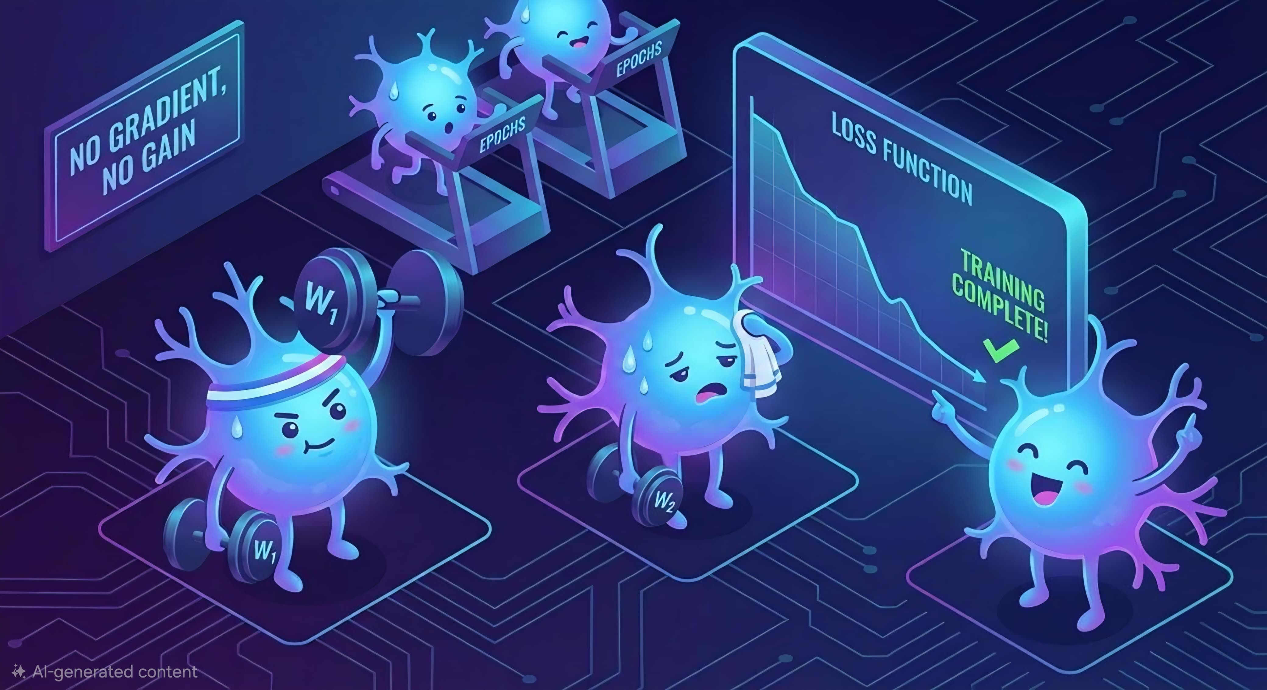
Part 0A: Neural Networks & The Learning Mechanism
Neural Networks & The Learning Mechanism
AI: Through an Architect’s Lens — Part 0A
Building deep intuition from first principles — how neural networks actually learn, explained step by step for engineers who want to truly understand the machinery before architecting with it.
Target Audience: Senior engineers building foundational ML understanding.
Prerequisites: Basic calculus (what a derivative means), linear algebra (matrix multiplication), Python (loops, functions, lists).
Reading Time: 90–120 minutes (take breaks — this is dense material).
Series Context: Foundation for Sequences & Transformers (Part 0B), then LLM Architecture (Part 1).
Code: https://github.com/phoenixtb/ai_through_architects_lens/tree/main/0A.
A Note on the Code Blocks. The code examples in this tutorial do more than demonstrate implementation — they tell stories. You’ll find ASCII diagrams, step-by-step narratives, and “why it matters” explanations embedded right in the output. Take a moment to read through the printed output, not just the code itself. That’s where much of the intuition lives.
Introduction: What Are We Actually Trying to Do?
Before we write a single equation, let’s be crystal clear about the problem we’re solving.
The Traditional Programming Paradigm
As software engineers, we’re trained to write explicit rules:
# Traditional programming: We write the rulesdef approve_loan(income, credit_score, employment_years): if credit_score < 600: return False # Rule 1: Bad credit = reject if income < 30000 and employment_years < 2: return False # Rule 2: Low income + short employment = reject if income > 100000: return True # Rule 3: High income = approve # ... hundreds more rulesThis works when:
- You can articulate the rules clearly
- The rules are relatively simple
- Edge cases are manageable
But what about:
- Detecting fraudulent transactions? (Patterns are subtle and constantly evolving)
- Recognizing faces in photos? (Try writing rules for “what makes a nose”)
- Understanding human language? (Grammar rules have more exceptions than rules)
The Machine Learning Paradigm
Machine learning flips the script:
Traditional: Human writes rules → Computer follows rules → OutputML: Human provides examples → Computer learns rules → OutputInstead of telling the computer how to decide, we show it examples of correct decisions and let it figure out the patterns.
# Machine learning paradigm: We provide examples, computer learns rulestraining_data = [ # (income, credit_score, employment_years) → approved? (75000, 720, 5, True), # This person was approved (25000, 580, 1, False), # This person was rejected (120000, 690, 3, True), # This person was approved (45000, 650, 8, True), # This person was approved # ... thousands more examples]model = learn_from_examples(training_data) # Computer figures out the rulesresult = model.predict(55000, 670, 4) # Apply learned rules to new caseThe key insight: We don’t program the solution. We program the learning process, then let the computer find the solution by studying examples.
What is a Neural Network?
A neural network is one specific architecture for learning from examples. It’s inspired by how biological brains work (loosely), but don’t get too hung up on the biology — it’s really just a mathematical structure that happens to be very good at finding patterns.
Think of it as a very flexible function:

Where function is not programmed by us — instead, it has millions of adjustable knobs (called parameters or weights), and the learning process figures out how to set those knobs so that function produces the right outputs for given inputs.
Now let’s understand how this actually works, starting with the smallest building block: the artificial neuron.
1. The Artificial Neuron: A Tiny Decision Maker
1.1 The Problem: Combining Multiple Factors into One Decision
Imagine you’re a loan officer at a bank. For each application, you receive:
- Annual income: €45,000
- Credit score: 680
- Years employed: 3
- Existing debt: €12,000
Your job: produce a single decision — approve or reject.
How do you mentally process this? Probably something like:
- Each factor matters, but not equally (credit score might matter more than years employed)
- You mentally “weigh” each factor by its importance
- You combine these weighted factors
- You compare against some internal threshold
- You decide: approve or reject This is exactly what an artificial neuron does.
1.2 Breaking Down the Neuron’s Components
Let’s build a neuron step by step:
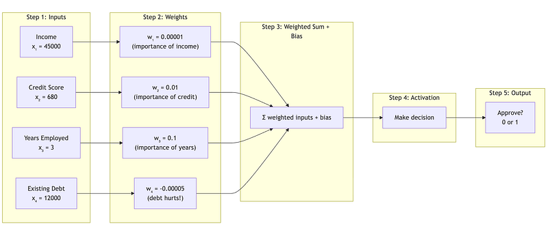
Component 1: Inputs (x)
These are the raw facts we’re given. In our loan example:

We typically write this as a vector:

Component 2: Weights (w)
Weights represent how important each input is to the decision. Higher weight = more influence.

Notice:
- Weights can be positive (feature helps) or negative (feature hurts)
- The magnitude reflects importance
- These numbers are NOT set by us — they’re LEARNED from training data Component 3: Bias (b)
The bias is like a baseline tendency. Think of it as:
- A positive bias means “lean toward approving”
- A negative bias means “lean toward rejecting”
For our example, let’s say

Component 4: Weighted Sum (z)
Now we combine everything. Each input gets multiplied by its weight, then we sum it all up and add the bias:

Let’s calculate:
Income contribution: 45000 × 0.00001 = 0.45Credit contribution: 680 × 0.01 = 6.80Employment contribution: 3 × 0.1 = 0.30Debt contribution: 12000 × -0.00005 = -0.60Bias: = -3.00─────────────────────────────────────────────────Total (z): = 3.95So z = 3.95. This is called the pre-activation value — the raw “score” before we make a decision. Component 5: Activation Function (σ)
The activation function converts our raw score into a decision. The simplest version:

Since z = 3.95 > 0, output = 1 (approve the loan).
1.3 The Complete Neuron in Code
Now let’s implement this with detailed comments:
import numpy as np
def single_neuron_step_by_step(inputs, weights, bias):    """    A single artificial neuron - the fundamental building block of neural networks.
    This function mimics how a loan officer might make a decision:                1. Consider multiple factors (inputs)                2. Weight each factor by its importance (weights)                3. Combine into a single score (weighted sum + bias)                4. Make a decision based on the score (activation)
    Parameters:                -----------    inputs : list or numpy array        The raw data we're making a decision about.        Example: [income, credit_score, years_employed, existing_debt]
    weights : list or numpy array        How important each input is. Learned during training.        Positive weight = input helps, Negative weight = input hurts        Example: [0.00001, 0.01, 0.1, -0.00005]
    bias : float        A baseline adjustment. Like a default tendency toward yes or no.        Positive bias = lean toward yes, Negative bias = lean toward no        Example: -3.0 (slightly conservative)
    Returns:                --------    tuple: (weighted_sum, pre_activation, output)                                - weighted_sum: The sum of (input × weight) for each input                                - pre_activation: weighted_sum + bias (the raw "score")                                - output: The final decision (1 or 0)    """
    # =========================================================================    # STEP 1: Calculate each input's contribution    # =========================================================================    # Each input contributes to the decision based on its weight.    # Think: "How much does this factor push toward yes or no?"
    contributions = []    print("Step 1: Calculate each input's contribution")    print("-" * 50)
    for i in range(len(inputs)):        # Multiply input by its weight to get its contribution        contribution = inputs[i] * weights[i]        contributions.append(contribution)
        # Explain what's happening        if weights[i] > 0:            direction = "pushes toward YES"        else:            direction = "pushes toward NO"
        print(f"  Input {i+1}: {inputs[i]:>10.2f} × weight {weights[i]:>10.5f} = {contribution:>8.2f} ({direction})")
    # =========================================================================    # STEP 2: Sum all contributions (weighted sum)    # =========================================================================    # Add up all the individual contributions to get a combined "evidence" score
    weighted_sum = sum(contributions)    print(f"\nStep 2: Sum all contributions")    print("-" * 50)    print(f"  Weighted sum = {weighted_sum:.2f}")
    # =========================================================================    # STEP 3: Add bias (pre-activation)    # =========================================================================    # The bias shifts our decision threshold.    # Positive bias = easier to say yes, Negative bias = harder to say yes
    pre_activation = weighted_sum + bias    print(f"\nStep 3: Add bias")    print("-" * 50)    print(f"  Pre-activation = weighted_sum + bias")    print(f"  Pre-activation = {weighted_sum:.2f} + ({bias:.2f}) = {pre_activation:.2f}")
    # =========================================================================    # STEP 4: Apply activation function (make decision)    # =========================================================================    # Convert the raw score into a final decision.    # Here we use a simple "step function": positive = yes, negative/zero = no
    if pre_activation > 0:        output = 1  # Approve        decision = "APPROVE (score > 0)"    else:        output = 0  # Reject        decision = "REJECT (score ≤ 0)"
    print(f"\nStep 4: Apply activation (decision rule)")    print("-" * 50)    print(f"  Rule: If pre-activation > 0, output 1 (yes), else output 0 (no)")    print(f"  {pre_activation:.2f} > 0? → {decision}")
    return weighted_sum, pre_activation, output

# =============================================================================# EXAMPLE: Loan approval decision# =============================================================================
print("=" * 60)print("LOAN APPROVAL NEURON EXAMPLE")print("=" * 60)print()
# Our applicant's datainputs = [    45000,   # Annual income (€)    680,     # Credit score (300-850 scale)    3,       # Years employed    12000    # Existing debt (€)]
# How important each factor is (these would be LEARNED in a real model)weights = [                0.00001,   # Income: small weight because numbers are large                0.01,      # Credit score: moderate importance                0.1,       # Years employed: some importance                -0.00005   # Existing debt: NEGATIVE because debt is bad]
# Baseline tendency (slightly conservative bank)bias = -3.0
print("Applicant data:")print(f"  Income: €{inputs[0]:,}")print(f"  Credit Score: {inputs[1]}")print(f"  Years Employed: {inputs[2]}")print(f"  Existing Debt: €{inputs[3]:,}")print()
# Run the neuronweighted_sum, pre_activation, output = single_neuron_step_by_step(inputs, weights, bias)
print()print("=" * 60)print(f"FINAL DECISION: {'APPROVED' if output == 1 else 'REJECTED'}")print("=" * 60)
Output:
============================================================LOAN APPROVAL NEURON EXAMPLE============================================================
Applicant data:  Income: €45,000  Credit Score: 680  Years Employed: 3  Existing Debt: €12,000
Step 1: Calculate each input's contribution--------------------------------------------------  Input 1:   45000.00 × weight    0.00001 =     0.45 (pushes toward YES)  Input 2:     680.00 × weight    0.01000 =     6.80 (pushes toward YES)  Input 3:       3.00 × weight    0.10000 =     0.30 (pushes toward YES)  Input 4:   12000.00 × weight   -0.00005 =    -0.60 (pushes toward NO)
Step 2: Sum all contributions--------------------------------------------------  Weighted sum = 6.95
Step 3: Add bias--------------------------------------------------  Pre-activation = weighted_sum + bias  Pre-activation = 6.95 + (-3.00) = 3.95
Step 4: Apply activation (decision rule)--------------------------------------------------  Rule: If pre-activation > 0, output 1 (yes), else output 0 (no)        3.95 > 0? → APPROVE (score > 0)
============================================================FINAL DECISION: APPROVED============================================================
1.4 The Mathematical Notation (Now It Makes Sense)
Now that you understand what’s happening, the mathematical notation becomes clear: The weighted sum:

Or in vector notation (more compact):


1.5 The Compact Implementation
Once you understand the concepts, we can write this more concisely:
import numpy as np
def neuron(x, w, b, activation_fn):    """    A single neuron in compact form.
    Parameters:                -----------    x : numpy array, shape (n_features,)        Input values    w : numpy array, shape (n_features,)        Weights (learned parameters)    b : float        Bias (learned parameter)    activation_fn : function        The activation function to apply
    Returns:                --------    float: The neuron's output    """    # np.dot computes the dot product (sum of element-wise products)    # This is the "weighted sum" step in one line    z = np.dot(w, x) + b
    # Apply activation function to get final output    y = activation_fn(z)
    return y

# Simple step activation functiondef step_activation(z):    """Return 1 if z > 0, else 0"""    return 1 if z > 0 else 0

# Example usagex = np.array([45000, 680, 3, 12000])w = np.array([0.00001, 0.01, 0.1, -0.00005])b = -3.0
output = neuron(x, w, b, step_activation)print(f"Output: {output}") # Output: 1 (approved) ---2. Why Activation Functions Matter: The Need for Non-Linearity
2.1 The Problem with Linear Combinations
Our simple step function works, but real neurons in neural networks use different activation functions. Why? Let’s understand the fundamental problem.

This is a linear combination — we’re just scaling inputs and adding them up. What if we stack two neurons?
Neuron 1: z₁ = w₁₁x₁ + w₁₂x₂ + b₁Neuron 2 (takes z₁ as input): z₂ = w₂₁z₁ + b₂Let’s substitute:
z₂ = w₂₁(w₁₁x₁ + w₁₂x₂ + b₁) + b₂ = w₂₁w₁₁x₁ + w₂₁w₁₂x₂ + w₂₁b₁ + b₂ = (w₂₁w₁₁)x₁ + (w₂₁w₁₂)x₂ + (w₂₁b₁ + b₂) = W₁x₁ + W₂x₂ + BThis is still just a linear combination! We could replace two neurons with one — the second neuron adds no new capability.
No matter how many linear neurons we stack, the result is always equivalent to a single linear transformation. This is useless for complex patterns.
2.2 Non-Linearity Breaks This Limitation
By inserting a non-linear function between layers, we break this collapse:
Neuron 1: z₁ = w₁₁x₁ + w₁₂x₂ + b₁          a₁ = σ(z₁)           ← Non-linear activation!
Neuron 2: z₂ = w₂₁a₁ + b₂      ← Now takes σ(z₁), not z₁          a₂ = σ(z₂)
Because σ is non-linear, we can’t simplify this to a single layer. Each additional layer adds representational power — the ability to capture more complex patterns.
2.3 Common Activation Functions
Let’s explore the most important activation functions: Sigmoid: Squashing to (0, 1)
The sigmoid function smoothly squashes any input to a value between 0 and 1:

import numpy as np
def sigmoid(z):    """    Sigmoid activation function.
    What it does:                - Takes any real number as input                - Outputs a value between 0 and 1                - Smooth, S-shaped curve
    When to use:                - Output layer for binary classification (probability of class 1)                - Historically used in hidden layers, but rarely now (see ReLU)
    Why it works:                - Large negative z → output ≈ 0                - Large positive z → output ≈ 1                - z = 0 → output = 0.5
    Problem:                - For very large or very small z, the gradient is nearly 0                - This causes "vanishing gradients" in deep networks (explained later)    """    return 1 / (1 + np.exp(-z))
# Examplesprint("Sigmoid examples:")print(f"  sigmoid(-10) = {sigmoid(-10):.6f}")  # ≈ 0 (very negative → near 0)print(f"  sigmoid(-2)  = {sigmoid(-2):.6f}")   # = 0.119print(f"  sigmoid(0)   = {sigmoid(0):.6f}")    # = 0.5 (midpoint)print(f"  sigmoid(2)   = {sigmoid(2):.6f}")    # = 0.881print(f"  sigmoid(10)  = {sigmoid(10):.6f}")   # ≈ 1 (very positive → near 1)
ReLU: The Modern Default
ReLU (Rectified Linear Unit) is beautifully simple — if the input is positive, pass it through; if negative, output zero:

def relu(z):    """    ReLU (Rectified Linear Unit) activation function.
    What it does:                - If z > 0, output z (pass through unchanged)                - If z ≤ 0, output 0 (block negative values)
    When to use:                - Default choice for hidden layers in modern networks                - Works well in deep networks
    Why it's great:                - Computationally efficient (just a comparison)                - Doesn't saturate for positive values (gradient = 1)                - Creates sparse representations (many zeros)
    Problem:                - "Dead neurons": If a neuron's output is always negative,      it will always output 0 and never update (gradient = 0)    """    return np.maximum(0, z)
# Examplesprint("\nReLU examples:")print(f"  relu(-10) = {relu(-10)}")   # 0 (negative → blocked)print(f"  relu(-2)  = {relu(-2)}")    # 0print(f"  relu(0)   = {relu(0)}")     # 0print(f"  relu(2)   = {relu(2)}")     # 2 (positive → passed through)print(f"  relu(10)  = {relu(10)}")    # 10
Softmax: Probability Distribution over Multiple Classes
When you need to choose between multiple classes (not just yes/no), softmax converts a vector of scores into probabilities:

def softmax(z):    """    Softmax activation function.
    What it does:                - Takes a vector of K raw scores (one per class)                - Converts to K probabilities that sum to 1                - Higher scores get higher probabilities
    When to use:                - Output layer for multi-class classification                - Example: Classifying images into 10 digit classes (0-9)
    Why it works:                - Exponential makes all values positive                - Division by sum ensures they add to 1                - Preserves ranking (highest score → highest probability)
    Note: We subtract max(z) for numerical stability to prevent    overflow when computing exp() of large numbers.    """    # Subtract max for numerical stability (doesn't change result)    exp_z = np.exp(z - np.max(z))    return exp_z / np.sum(exp_z)
# Example: Classifying a digit image# Raw scores from a network for classes 0-9scores = np.array([1.2, 0.5, 0.1, 3.8, 0.2, 0.1, 0.3, 0.9, 0.4, 0.2])
probabilities = softmax(scores)print("\nSoftmax example (digit classification):")print("Raw scores:", scores)print("Probabilities:", np.round(probabilities, 3))print(f"Sum of probabilities: {np.sum(probabilities):.6f}")  # Should be 1.0print(f"Predicted class: {np.argmax(probabilities)} (highest probability)")
2.4 Activation Function Decision Guide
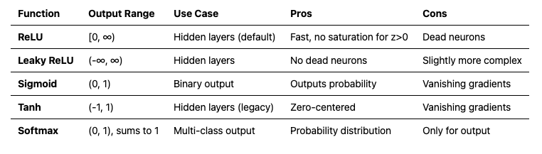
Practical rule: Use ReLU in hidden layers, sigmoid for binary output, softmax for multi-class output.
3. Building Networks: Stacking Layers
3.1 Why One Neuron Isn’t Enough
A single neuron can only learn linear decision boundaries — it divides the input space with a straight line (or hyperplane in higher dimensions).
Single neuron decision boundary:
    Credit Score         ↑         |      ✓ ✓ ✓ ✓         |    ✓ ✓ ✓ ✓ ✓         |  ─────────────── ← Linear boundary         |  ✗ ✗ ✗ ✗         |✗ ✗ ✗ ✗ ✗         └──────────────→ Income
But real-world patterns are rarely linear:
Real fraud detection patterns:
    Transaction Amount         ↑         |    ✓   ✗ ✗   ✓         |  ✓ ✓ ✗ ✗ ✗ ✓ ✓         |    ✓ ✗ ✗ ✗ ✓    ← Can't separate with a line!         |      ✓ ✓ ✓         |        ✓         └──────────────→ Transaction Time
3.2 Layers: Groups of Neurons Working Together
A layer is a group of neurons that all receive the same inputs but have different weights. Each neuron in a layer learns to detect a different pattern.
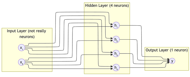
In this network:
- Input layer: 2 features (not actual neurons — just the raw data)
- Hidden layer: 4 neurons, each detecting a different pattern
- Output layer: 1 neuron, combining the patterns into a final decision
Why “hidden”? We don’t directly observe what hidden layers compute — they learn internal representations automatically.
3.3 What Each Layer Learns
Here’s the magic: each layer learns progressively more abstract features.
In image recognition:
- Layer 1: Edges (horizontal, vertical, diagonal lines)
- Layer 2: Shapes (corners, curves, simple textures)
- Layer 3: Parts (eyes, noses, wheels)
- Layer 4: Objects (faces, cars, dogs)
In fraud detection:
- Layer 1: Basic patterns (transaction size, time of day)
- Layer 2: Combinations (large late-night transactions)
- Layer 3: Behavioral patterns (sudden change in spending location)
- Layer 4: Fraud signature (combination of suspicious patterns)
This is why depth matters. Shallow networks can only learn simple patterns. Deep networks can build complex hierarchical representations.
3.4 The Forward Pass: Computing Outputs Layer by Layer
Let’s trace through a complete forward pass:
import numpy as np
class SimpleNetwork:    """    A simple 2-layer neural network for binary classification.
    Architecture: Input → Hidden Layer (ReLU) → Output Layer (Sigmoid)
    This network can learn non-linear decision boundaries because:                1. The hidden layer creates multiple non-linear features                2. The output layer combines them for the final decision    """
    def __init__(self, input_size, hidden_size, output_size):        """        Initialize the network with random weights.
        Parameters:                                -----------        input_size : int            Number of input features (e.g., 2 for [income, credit_score])        hidden_size : int            Number of neurons in hidden layer (more = more capacity)        output_size : int            Number of output neurons (1 for binary classification)        """        # =====================================================================        # Weight Initialization        # =====================================================================        # Weights connect neurons between layers.        # Shape: (neurons_in_this_layer, neurons_in_previous_layer)        #        # We initialize with small random values. The scaling factor        # (np.sqrt(2/n)) is called "He initialization" and helps training.        # We'll explain WHY this matters in the training section.
        # Hidden layer weights: connects input to hidden        # Shape: (hidden_size, input_size) = (4, 2) if hidden=4, input=2        self.W1 = np.random.randn(hidden_size, input_size) * np.sqrt(2.0 / input_size)
        # Hidden layer biases: one per hidden neuron        # Shape: (hidden_size, 1) = (4, 1)        self.b1 = np.zeros((hidden_size, 1))
        # Output layer weights: connects hidden to output        # Shape: (output_size, hidden_size) = (1, 4)        self.W2 = np.random.randn(output_size, hidden_size) * np.sqrt(2.0 / hidden_size)
        # Output layer biases: one per output neuron        # Shape: (output_size, 1) = (1, 1)        self.b2 = np.zeros((output_size, 1))
        print(f"Network initialized:")        print(f"  Input size: {input_size}")        print(f"  Hidden size: {hidden_size}")        print(f"  Output size: {output_size}")        print(f"  W1 shape: {self.W1.shape} (hidden × input)")        print(f"  b1 shape: {self.b1.shape}")        print(f"  W2 shape: {self.W2.shape} (output × hidden)")        print(f"  b2 shape: {self.b2.shape}")        print(f"  Total parameters: {self.W1.size + self.b1.size + self.W2.size + self.b2.size}")
    def forward(self, X, verbose=False):        """        Forward pass: compute output given input.
        Parameters:                                -----------        X : numpy array, shape (input_size, batch_size)            Input data. Each column is one example.            Example: shape (2, 32) = 2 features, 32 examples
        verbose : bool            If True, print intermediate steps
        Returns:                                --------        numpy array, shape (output_size, batch_size)            Output predictions (probabilities for each example)        """        if verbose:            print("\n" + "="*60)            print("FORWARD PASS")            print("="*60)            print(f"\nInput X shape: {X.shape}")            print(f"Input X:\n{X}")
        # =====================================================================        # LAYER 1: Input → Hidden        # =====================================================================
        # Step 1a: Compute weighted sum for hidden layer        # Z1 = W1 @ X + b1        # Matrix multiplication: (hidden, input) @ (input, batch) = (hidden, batch)        # This computes ALL hidden neurons for ALL examples at once!        Z1 = np.dot(self.W1, X) + self.b1
        if verbose:            print(f"\n--- Layer 1 (Input → Hidden) ---")            print(f"W1 @ X + b1 = Z1")            print(f"({self.W1.shape}) @ ({X.shape}) + ({self.b1.shape}) = ({Z1.shape})")            print(f"Z1 (pre-activation):\n{Z1}")
        # Step 1b: Apply ReLU activation        # ReLU(z) = max(0, z) for each element        A1 = np.maximum(0, Z1)
        if verbose:            print(f"A1 = ReLU(Z1):\n{A1}")
        # =====================================================================        # LAYER 2: Hidden → Output        # =====================================================================
        # Step 2a: Compute weighted sum for output layer        Z2 = np.dot(self.W2, A1) + self.b2
        if verbose:            print(f"\n--- Layer 2 (Hidden → Output) ---")            print(f"W2 @ A1 + b2 = Z2")            print(f"({self.W2.shape}) @ ({A1.shape}) + ({self.b2.shape}) = ({Z2.shape})")            print(f"Z2 (pre-activation):\n{Z2}")
        # Step 2b: Apply sigmoid activation        # Sigmoid squashes to (0, 1) for probability output        A2 = 1 / (1 + np.exp(-Z2))
        if verbose:            print(f"A2 = sigmoid(Z2):\n{A2}")            print(f"\nFinal output shape: {A2.shape}")            print(f"Predictions (probabilities): {A2.flatten()}")
        # Store intermediate values (needed for backpropagation later)        self.cache = {            'X': X, 'Z1': Z1, 'A1': A1, 'Z2': Z2, 'A2': A2        }
        return A2

# =============================================================================# EXAMPLE: Forward pass demonstration# =============================================================================
print("="*70)print("FORWARD PASS DEMONSTRATION")print("="*70)
# Create a small networknp.random.seed(42)  # For reproducible resultsnet = SimpleNetwork(input_size=2, hidden_size=4, output_size=1)
# Create sample input: 3 loan applications# Each column is one application: [income (scaled), credit_score (scaled)]X = np.array([    [0.45, 0.80, 0.25],   # Incomes (scaled to ~0-1)    [0.68, 0.90, 0.55]    # Credit scores (scaled to ~0-1)])
print("\n" + "="*70)print("Processing 3 loan applications...")print("="*70)
# Run forward pass with detailed outputpredictions = net.forward(X, verbose=True)
print("\n" + "="*70)print("INTERPRETATION")print("="*70)print(f"Application 1 (income=0.45, credit=0.68): {predictions[0,0]:.1%} approval probability")print(f"Application 2 (income=0.80, credit=0.90): {predictions[0,1]:.1%} approval probability")print(f"Application 3 (income=0.25, credit=0.55): {predictions[0,2]:.1%} approval probability")Output:
======================================================================FORWARD PASS DEMONSTRATION======================================================================Network initialized:  Input size: 2  Hidden size: 4  Output size: 1  W1 shape: (4, 2) (hidden × input)  b1 shape: (4, 1)  W2 shape: (1, 4) (output × hidden)  b2 shape: (1, 1)  Total parameters: 17
======================================================================Processing 3 loan applications...======================================================================
============================================================FORWARD PASS============================================================
Input X shape: (2, 3)Input X:[[0.45 0.8  0.25] [0.68 0.9  0.55]]    --- Layer 1 (Input → Hidden) ---W1 @ X + b1 = Z1((4, 2)) @ ((2, 3)) + ((4, 1)) = ((4, 3))Z1 (pre-activation):[[ 0.12950164  0.27293345  0.04813317] [ 1.32712014  1.8888777   0.99958856] [-0.26458215 -0.39804596 -0.18731367] [ 1.23250138  1.95406151  0.8168923 ]]A1 = ReLU(Z1):[[0.12950164 0.27293345 0.04813317] [1.32712014 1.8888777  0.99958856] [0.         0.         0.        ] [1.23250138 1.95406151 0.8168923 ]]    --- Layer 2 (Hidden → Output) ---W2 @ A1 + b2 = Z2((1, 4)) @ ((4, 3)) + ((1, 1)) = ((1, 3))Z2 (pre-activation):[[ 0.06026819 -0.00945422  0.09849182]]A2 = sigmoid(Z2):[[0.51506249 0.49763646 0.52460307]]
Final output shape: (1, 3)Predictions (probabilities): [0.51506249 0.49763646 0.52460307]
======================================================================INTERPRETATION======================================================================Application 1 (income=0.45, credit=0.68): 51.5% approval probabilityApplication 2 (income=0.80, credit=0.90): 49.8% approval probabilityApplication 3 (income=0.25, credit=0.55): 52.5% approval probability
3.5 Key Insight: Matrix Operations Do Everything in Parallel
Notice how we process all examples at once using matrix multiplication. This is crucial for efficiency:
Instead of:    for each example:        for each neuron:            compute weighted sum
We do:    Z = W @ X + b  (one matrix operation, processes everything)
This parallelism is why GPUs (designed for matrix operations) excel at neural network training.
4. Loss Functions: Measuring How Wrong We Are
The network makes predictions. But how do we know if they’re good? We need a way to measure error — this is the loss function.
4.1 The Role of the Loss Function
The loss function (also called cost function or objective function) serves three purposes:
- Quantifies error: Converts “prediction was wrong” into a number
- Guides learning: Tells us which direction to adjust weights
- Enables comparison: Lower loss = better model Critical property: The loss must be differentiable (we can compute its gradient). This is how we’ll figure out which direction to adjust weights.
4.2 Mean Squared Error (MSE) for Regression
When predicting continuous values (house prices, temperatures), we use MSE:

def mean_squared_error(y_true, y_pred):    """    Mean Squared Error loss for regression problems.
    How it works:                1. For each prediction, compute error: (actual - predicted)                2. Square each error (makes all errors positive, penalizes big errors more)                3. Average across all examples
    Parameters:                -----------    y_true : numpy array        Actual values (ground truth)    y_pred : numpy array        Model's predictions
    Returns:                --------    float : The average squared error
    Example:                --------    Predicting house prices (in $100,000s):    Actual:    [3.0, 4.5, 2.0]  ($300K, $450K, $200K)    Predicted: [2.8, 4.2, 2.5]  ($280K, $420K, $250K)
    Errors:    [0.2, 0.3, -0.5]    Squared:   [0.04, 0.09, 0.25]    MSE:       0.1267
    Interpretation: On average, our squared error is 0.127, meaning    typical error is roughly sqrt(0.127) ≈ 0.36 ($36,000)    """    # Step 1: Compute errors    errors = y_true - y_pred
    # Step 2: Square the errors    # This makes negative errors positive AND penalizes large errors more    squared_errors = errors ** 2
    # Step 3: Average across all examples    mse = np.mean(squared_errors)
    return mse

# Example: House price predictiony_true = np.array([3.0, 4.5, 2.0])  # Actual pricesy_pred = np.array([2.8, 4.2, 2.5])  # Predicted prices
mse = mean_squared_error(y_true, y_pred)print(f"MSE: {mse:.4f}")print(f"Typical error magnitude: ${np.sqrt(mse) * 100000:,.0f}")
Why square the errors?
- Makes all errors positive (can’t have negative and positive errors cancel out)
- Penalizes large errors more heavily (error of 2 costs 4×, not 2×)
4.3 Binary Cross-Entropy for Classification
When predicting probabilities (spam/not spam, approve/reject), we use binary cross-entropy:

This looks complicated, but the intuition is simple:
def binary_cross_entropy(y_true, y_pred, epsilon=1e-15):    """    Binary Cross-Entropy loss for binary classification.
    How it works:                - If true label is 1, we want predicted probability to be HIGH      Loss = -log(predicted). If predicted=0.9, loss=-log(0.9)=0.1 (low, good!)                              If predicted=0.1, loss=-log(0.1)=2.3 (high, bad!)                    - If true label is 0, we want predicted probability to be LOW      Loss = -log(1-predicted). If predicted=0.1, loss=-log(0.9)=0.1 (low, good!)                                If predicted=0.9, loss=-log(0.1)=2.3 (high, bad!)
    Key insight: The -log function heavily penalizes confident WRONG predictions.                - Predicting 0.99 when true label is 0 → loss ≈ 4.6 (very bad!)                - Predicting 0.51 when true label is 0 → loss ≈ 0.7 (not great, but not terrible)
    This encourages the model to only be confident when it's right.
    Parameters:                -----------    y_true : numpy array        Actual labels (0 or 1)    y_pred : numpy array        Predicted probabilities (between 0 and 1)    epsilon : float        Small value to prevent log(0) which is undefined
    Returns:                --------    float : The average binary cross-entropy loss    """    # Clip predictions to prevent log(0) or log(1)    # log(0) = -infinity, which would break our computation    y_pred = np.clip(y_pred, epsilon, 1 - epsilon)
    # Compute loss for each example    # When y_true=1: loss = -log(y_pred)    # When y_true=0: loss = -log(1 - y_pred)    # This formula handles both cases elegantly:    individual_losses = -(        y_true * np.log(y_pred) +           # Active when y_true=1        (1 - y_true) * np.log(1 - y_pred)   # Active when y_true=0    )
    # Average across all examples    bce = np.mean(individual_losses)
    return bce

# Example: Loan approval classificationprint("Binary Cross-Entropy Examples:")print("-" * 50)
# Case 1: Correct and confident predictiony_true = np.array([1])       # Should be approvedy_pred = np.array([0.95])    # Model is confident: 95% approvalloss = binary_cross_entropy(y_true, y_pred)print(f"True=1, Pred=0.95 (confident, correct): Loss = {loss:.4f}")
# Case 2: Correct but uncertain predictiony_pred = np.array([0.55])    # Model is uncertain: 55% approvalloss = binary_cross_entropy(y_true, y_pred)print(f"True=1, Pred=0.55 (uncertain, correct): Loss = {loss:.4f}")
# Case 3: Wrong and confident prediction (VERY BAD)y_pred = np.array([0.05])    # Model is confident it should be rejected!loss = binary_cross_entropy(y_true, y_pred)print(f"True=1, Pred=0.05 (confident, WRONG): Loss = {loss:.4f}")
print()print("Notice: Confident wrong predictions have MUCH higher loss!")print("This teaches the model to be uncertain when it doesn't know.")
4.4 Why These Specific Loss Functions?
The choice isn’t arbitrary. These loss functions are mathematically well-suited for their tasks:

Don’t worry if the statistical justification isn’t clear — the practical rules are:
- Predicting a number? → Use MSE (or MAE if outliers are a concern)
- Predicting yes/no? → Use Binary Cross-Entropy with sigmoid output
- Predicting one of K classes? → Use Categorical Cross-Entropy with softmax output
5. Backpropagation: Teaching the Network
We can now:
- Make predictions (forward pass)
- Measure how wrong we are (loss function)
But how do we actually improve? We need to adjust the weights so the loss decreases. This is where backpropagation comes in.
5.1 The Core Idea: Follow the Gradient Downhill
Imagine you’re blindfolded on a hilly landscape, trying to find the lowest point:
- You can feel the slope under your feet
- You take a step in the downhill direction
- Repeat until you can’t go lower
This is gradient descent. The gradient tells us the direction of steepest ascent, so we go the opposite direction (descent).

The minus sign handles both cases automatically!
5.2 The Chain Rule: The Mathematical Foundation


In words: “The rate of change of y with respect to x equals the rate of change of y with respect to g, times the rate of change of g with respect to x.”
For neural networks, the computation graph looks like:
Input → [W1] → Z1 → [ReLU] → A1 → [W2] → Z2 → [Sigmoid] → A2 → [Loss] → LTo find how L depends on W1, we chain through all the intermediate steps:

5.3 Backpropagation Step by Step
Let’s trace through backpropagation on a simple 2-layer network. I’ll use concrete numbers so you can follow along.
import numpy as np
def backprop_step_by_step():    """    Demonstrate backpropagation with concrete numbers.
    Network: 2 inputs → 2 hidden neurons → 1 output    """    np.random.seed(42)
    print("="*70)    print("BACKPROPAGATION STEP BY STEP")    print("="*70)
    # =========================================================================    # SETUP: Define a simple network with known weights    # =========================================================================
    # Network architecture: 2 → 2 → 1
    # Hidden layer weights (2 neurons, each receiving 2 inputs)    W1 = np.array([        [0.1, 0.2],   # Neuron 1 weights        [0.3, 0.4]    # Neuron 2 weights    ])    b1 = np.array([[0.1], [0.2]])  # Biases for hidden neurons
    # Output layer weights (1 neuron receiving 2 inputs from hidden)    W2 = np.array([[0.5, 0.6]])  # Single output neuron    b2 = np.array([[0.3]])       # Bias for output
    print("\n--- NETWORK PARAMETERS ---")    print(f"W1 (hidden layer weights):\n{W1}")    print(f"b1 (hidden layer biases): {b1.flatten()}")    print(f"W2 (output layer weights): {W2}")    print(f"b2 (output layer bias): {b2.flatten()}")
    # =========================================================================    # INPUT DATA    # =========================================================================
    # Single training example    X = np.array([[0.5], [0.8]])  # Input features    Y = np.array([[1.0]])          # True label (should output 1)
    print(f"\n--- INPUT ---")    print(f"X (input features): {X.flatten()}")    print(f"Y (true label): {Y.flatten()}")
    # =========================================================================    # FORWARD PASS (compute predictions)    # =========================================================================
    print("\n" + "="*70)    print("FORWARD PASS")    print("="*70)
    # --- Hidden Layer ---    # Z1 = W1 @ X + b1    Z1 = np.dot(W1, X) + b1    print(f"\n[Hidden Layer] Z1 = W1 @ X + b1")    print(f"  W1 @ X = {W1} @ {X.flatten()} = {np.dot(W1, X).flatten()}")    print(f"  Z1 = {np.dot(W1, X).flatten()} + {b1.flatten()} = {Z1.flatten()}")
    # Apply ReLU: A1 = max(0, Z1)    A1 = np.maximum(0, Z1)    print(f"\n[Hidden Layer] A1 = ReLU(Z1) = max(0, Z1)")    print(f"  A1 = max(0, {Z1.flatten()}) = {A1.flatten()}")
    # --- Output Layer ---    # Z2 = W2 @ A1 + b2    Z2 = np.dot(W2, A1) + b2    print(f"\n[Output Layer] Z2 = W2 @ A1 + b2")    print(f"  Z2 = {W2} @ {A1.flatten()} + {b2.flatten()} = {Z2.flatten()}")
    # Apply Sigmoid: A2 = 1 / (1 + exp(-Z2))    A2 = 1 / (1 + np.exp(-Z2))    print(f"\n[Output Layer] A2 = sigmoid(Z2)")    print(f"  A2 = sigmoid({Z2.flatten()}) = {A2.flatten()}")
    # --- Compute Loss ---    # Binary Cross-Entropy: L = -[Y*log(A2) + (1-Y)*log(1-A2)]    epsilon = 1e-15    L = -np.mean(Y * np.log(A2 + epsilon) + (1 - Y) * np.log(1 - A2 + epsilon))    print(f"\n[Loss] Binary Cross-Entropy")    print(f"  L = {L:.6f}")    print(f"  Interpretation: Predicted {A2[0,0]:.4f}, true label is {Y[0,0]}")    print(f"  Error: We predicted {A2[0,0]:.1%} probability, should be {Y[0,0]:.0%}")
    # =========================================================================    # BACKWARD PASS (compute gradients)    # =========================================================================
    print("\n" + "="*70)    print("BACKWARD PASS")    print("="*70)    print("\nWe now compute: How does changing each weight affect the loss?")
    m = 1  # Number of examples (batch size)
    # --- Step 1: Gradient of Loss w.r.t. A2 ---    # For BCE: dL/dA2 = -Y/A2 + (1-Y)/(1-A2)    dL_dA2 = -(Y / (A2 + epsilon)) + (1 - Y) / (1 - A2 + epsilon)    print(f"\n[Step 1] Gradient of Loss w.r.t. Output (dL/dA2)")    print(f"  Formula: dL/dA2 = -Y/A2 + (1-Y)/(1-A2)")    print(f"  dL/dA2 = {dL_dA2.flatten()[0]:.6f}")    print(f"  Meaning: If we increase A2 slightly, loss changes by this amount")
    # --- Step 2: Gradient through Sigmoid ---    # Sigmoid derivative: dA2/dZ2 = A2 * (1 - A2)    dA2_dZ2 = A2 * (1 - A2)    dL_dZ2 = dL_dA2 * dA2_dZ2  # Chain rule!    print(f"\n[Step 2] Chain through Sigmoid (dL/dZ2 = dL/dA2 × dA2/dZ2)")    print(f"  Sigmoid derivative: dA2/dZ2 = A2 × (1-A2) = {A2[0,0]:.4f} × {1-A2[0,0]:.4f} = {dA2_dZ2[0,0]:.6f}")    print(f"  Chain rule: dL/dZ2 = {dL_dA2[0,0]:.6f} × {dA2_dZ2[0,0]:.6f} = {dL_dZ2[0,0]:.6f}")
    # --- Step 3: Gradients for Output Layer Weights ---    # dL/dW2 = dL/dZ2 × dZ2/dW2 = dL/dZ2 × A1    dL_dW2 = np.dot(dL_dZ2, A1.T) / m    dL_db2 = np.sum(dL_dZ2, axis=1, keepdims=True) / m    print(f"\n[Step 3] Gradients for Output Layer (W2, b2)")    print(f"  dL/dW2 = dL/dZ2 × A1ᵀ = {dL_dZ2[0,0]:.6f} × {A1.flatten()} = {dL_dW2.flatten()}")    print(f"  dL/db2 = dL/dZ2 = {dL_db2.flatten()}")    print(f"  Meaning: These tell us how to adjust W2 and b2 to reduce loss")
    # --- Step 4: Backpropagate to Hidden Layer ---    # dL/dA1 = W2ᵀ × dL/dZ2    dL_dA1 = np.dot(W2.T, dL_dZ2)    print(f"\n[Step 4] Backpropagate error to Hidden Layer (dL/dA1)")    print(f"  dL/dA1 = W2ᵀ × dL/dZ2 = {W2.T.flatten()} × {dL_dZ2[0,0]:.6f} = {dL_dA1.flatten()}")    print(f"  Meaning: This is how much each hidden neuron contributed to the error")
    # --- Step 5: Gradient through ReLU ---    # ReLU derivative: 1 if Z1 > 0, else 0    dA1_dZ1 = (Z1 > 0).astype(float)  # 1 where Z1 > 0, else 0    dL_dZ1 = dL_dA1 * dA1_dZ1  # Chain rule    print(f"\n[Step 5] Chain through ReLU (dL/dZ1 = dL/dA1 × dA1/dZ1)")    print(f"  ReLU derivative: dA1/dZ1 = {dA1_dZ1.flatten()} (1 if Z1>0, else 0)")    print(f"  dL/dZ1 = {dL_dA1.flatten()} × {dA1_dZ1.flatten()} = {dL_dZ1.flatten()}")
    # --- Step 6: Gradients for Hidden Layer Weights ---    dL_dW1 = np.dot(dL_dZ1, X.T) / m    dL_db1 = np.sum(dL_dZ1, axis=1, keepdims=True) / m    print(f"\n[Step 6] Gradients for Hidden Layer (W1, b1)")    print(f"  dL/dW1 = dL/dZ1 × Xᵀ:")    print(f"    {dL_dW1}")    print(f"  dL/db1 = {dL_db1.flatten()}")
    # =========================================================================    # WEIGHT UPDATE    # =========================================================================
    print("\n" + "="*70)    print("WEIGHT UPDATE (Gradient Descent)")    print("="*70)
    learning_rate = 0.1    print(f"\nLearning rate: {learning_rate}")    print(f"Update rule: W_new = W_old - learning_rate × gradient")
    W2_new = W2 - learning_rate * dL_dW2    b2_new = b2 - learning_rate * dL_db2    W1_new = W1 - learning_rate * dL_dW1    b1_new = b1 - learning_rate * dL_db1
    print(f"\nW2: {W2.flatten()} → {W2_new.flatten()}")    print(f"b2: {b2.flatten()} → {b2_new.flatten()}")    print(f"W1:\n{W1} →\n{W1_new}")    print(f"b1: {b1.flatten()} → {b1_new.flatten()}")
    # =========================================================================    # VERIFY IMPROVEMENT    # =========================================================================
    print("\n" + "="*70)    print("VERIFY: Did the update help?")    print("="*70)
    # Forward pass with new weights    Z1_new = np.dot(W1_new, X) + b1_new    A1_new = np.maximum(0, Z1_new)    Z2_new = np.dot(W2_new, A1_new) + b2_new    A2_new = 1 / (1 + np.exp(-Z2_new))    L_new = -np.mean(Y * np.log(A2_new + epsilon) + (1 - Y) * np.log(1 - A2_new + epsilon))
    print(f"\nBefore update:")    print(f"  Prediction: {A2[0,0]:.4f} (target: {Y[0,0]:.1f})")    print(f"  Loss: {L:.6f}")
    print(f"\nAfter update:")    print(f"  Prediction: {A2_new[0,0]:.4f} (target: {Y[0,0]:.1f})")    print(f"  Loss: {L_new:.6f}")
    print(f"\nImprovement: Loss decreased by {L - L_new:.6f} ({(L-L_new)/L*100:.1f}%)")    print("The prediction moved closer to the target! 🎉")
    return {        'W1': W1_new, 'b1': b1_new, 'W2': W2_new, 'b2': b2_new,        'final_loss': L_new    }

# Run the demonstrationresult = backprop_step_by_step()
5.4 The Key Insight: Blame Assignment
Backpropagation is essentially a blame assignment algorithm:
- Output layer: Directly responsible for the prediction → gets gradient directly from loss
- Hidden layer: Contributed to the output → gets “blamed” in proportion to how much it influenced the output (through W2)
- Earlier layers: Even more indirect blame assignment
The chain rule distributes “blame” (gradients) backwards through the network, and each weight is updated in proportion to how much it contributed to the error.
6. Optimization: Taking the Right Steps
We know the direction to move (gradient). Now we need to decide how far to step.
6.1 Learning Rate: The Critical Hyperparameter

Too small: Progress is painfully slow. May take forever to converge. Too large: Overshoots the minimum. May oscillate wildly or diverge.
def learning_rate_demo():    """    Demonstrate the effect of learning rate.
    We'll minimize a simple function: f(x) = x²    The minimum is at x = 0.    """
    def f(x):        return x ** 2
    def gradient(x):        return 2 * x  # Derivative of x²
    print("="*60)    print("LEARNING RATE COMPARISON")    print("="*60)    print("Minimizing f(x) = x², starting at x = 10")    print("Optimal solution: x = 0")    print()
    learning_rates = [0.01, 0.1, 0.5, 0.9, 5.0]
    for lr in learning_rates:        x = 10.0  # Starting point        history = [x]
        print(f"Learning rate = {lr}:")
        for step in range(20):            grad = gradient(x)            x = x - lr * grad  # Gradient descent update            history.append(x)
            # Check for divergence            if abs(x) > 1e10:                print(f"  Step {step+1}: DIVERGED! (x = {x:.2e})")                break        else:            print(f"  After 20 steps: x = {x:.6f}, f(x) = {f(x):.6f}")
        # Categorize behavior        if abs(x) > 1e10:            print(f"  Result: DIVERGED (learning rate too high)")        elif abs(x) < 0.01:            print(f"  Result: CONVERGED (good learning rate)")        else:            print(f"  Result: STILL CONVERGING (learning rate may be too low)")        print()

learning_rate_demo()
6.2 Adam: The Practical Default
Plain gradient descent has issues:
- Same learning rate for all parameters (some may need bigger/smaller steps)
- Easily stuck in flat regions
- Oscillates in narrow valleys Adam (Adaptive Moment Estimation) fixes these issues by:
- Keeping a running average of gradients (momentum)
- Keeping a running average of squared gradients (adaptive learning rates)
class AdamOptimizer:    """    Adam optimizer - the practical default for most neural networks.
    Key ideas:                1. Momentum: Keep a running average of past gradients.       If gradients consistently point the same direction, speed up.       This helps escape flat regions and smooth out noise.                    2. Adaptive learning rates: Keep track of how much each parameter's       gradient varies. Parameters with wildly varying gradients get       smaller learning rates. Parameters with consistent gradients       get larger learning rates.
    Default hyperparameters (rarely need changing):                - learning_rate = 0.001                - beta1 = 0.9 (momentum decay)                - beta2 = 0.999 (squared gradient decay)                - epsilon = 1e-8 (prevents division by zero)    """
    def __init__(self, learning_rate=0.001, beta1=0.9, beta2=0.999, epsilon=1e-8):        """        Parameters:                                -----------        learning_rate : float            Base step size. 0.001 is good for most problems.
        beta1 : float            Decay rate for first moment (gradient average).                                                0.9 means "remember 90% of past gradients".
        beta2 : float            Decay rate for second moment (squared gradient average).                                                0.999 means "remember 99.9% of past squared gradients".
        epsilon : float            Small constant to prevent division by zero.        """        self.lr = learning_rate        self.beta1 = beta1        self.beta2 = beta2        self.epsilon = epsilon
        # These store running averages for each parameter        self.m = {}  # First moment (gradient average)        self.v = {}  # Second moment (squared gradient average)        self.t = 0   # Timestep counter
    def update(self, params, grads):        """        Update parameters using Adam algorithm.
        Parameters:                                -----------        params : dict            Dictionary of parameters, e.g., {'W1': array, 'b1': array, ...}        grads : dict            Dictionary of gradients, e.g., {'dW1': array, 'db1': array, ...}        """        self.t += 1  # Increment timestep
        for key in params:            # Get gradient for this parameter            # Convert 'W1' to 'dW1', 'b1' to 'db1', etc.            grad_key = 'd' + key            if grad_key not in grads:                continue
            grad = grads[grad_key]
            # Initialize moments on first update            if key not in self.m:                self.m[key] = np.zeros_like(params[key])                self.v[key] = np.zeros_like(params[key])
            # ================================================================            # Step 1: Update first moment (momentum)            # ================================================================            # m = β₁ × m + (1 - β₁) × gradient            # This is a weighted average of past gradients            self.m[key] = self.beta1 * self.m[key] + (1 - self.beta1) * grad
            # ================================================================            # Step 2: Update second moment (adaptive learning rate)            # ================================================================            # v = β₂ × v + (1 - β₂) × gradient²            # This tracks how much the gradient varies            self.v[key] = self.beta2 * self.v[key] + (1 - self.beta2) * (grad ** 2)
            # ================================================================            # Step 3: Bias correction            # ================================================================            # The moments are biased toward zero initially (they start at 0)            # This correction compensates for that bias            m_corrected = self.m[key] / (1 - self.beta1 ** self.t)****            v_corrected = self.v[key] / (1 - self.beta2 ** self.t)
            # ================================================================            # Step 4: Update parameter            # ================================================================            # The key insight: we divide by sqrt(v), which gives each parameter            # its own effective learning rate based on gradient history            params[key] -= self.lr * m_corrected / (np.sqrt(v_corrected) + self.epsilon)
Driver forthe Adam optimizer:
import numpy as npdef adam_demo():    """    Compare Adam vs vanilla gradient descent on f(x) = x²    """    def f(x):        return x ** 2
    def gradient(x):        return 2 * x
    print("="*60)    print("ADAM vs VANILLA GRADIENT DESCENT")    print("="*60)    print("Minimizing f(x) = x², starting at x = 10\n")
    # Vanilla GD with a conservative learning rate    x_gd = 10.0    lr = 0.1    gd_history = [x_gd]
    for _ in range(20):        x_gd = x_gd - lr * gradient(x_gd)        gd_history.append(x_gd)
    # Adam optimizer    x_adam = 10.0    adam = AdamOptimizer(learning_rate=0.5)  # Can use larger lr with Adam    adam_history = [x_adam]
    for _ in range(20):        # Adam expects dict format, we'll simulate it        params = {'x': np.array([x_adam])}        grads = {'dx': np.array([gradient(x_adam)])}        adam.update(params, grads)        x_adam = params['x'][0]        adam_history.append(x_adam)
    print(f"Vanilla GD (lr={lr}):")    print(f"  Step 5:  x = {gd_history[5]:.6f}")    print(f"  Step 10: x = {gd_history[10]:.6f}")    print(f"  Step 20: x = {gd_history[20]:.6f}")    print()    print(f"Adam (lr=0.5):")    print(f"  Step 5:  x = {adam_history[5]:.6f}")    print(f"  Step 10: x = {adam_history[10]:.6f}")    print(f"  Step 20: x = {adam_history[20]:.6f}")    print()    print("Adam adapts its effective learning rate based on gradient history.")
adam_demo()
6.3 Optimizer Selection Guide

Practical advice: Start with Adam at lr=0.001. Adjust only if:
- Training is unstable → decrease learning rate
- Training is too slow → try increasing learning rate
-
Loss plateaus early → try learning rate schedule
7. Practical Training Concerns
Understanding theory is necessary but not sufficient. Here are the practical challenges you’ll face.
7.1 Vanishing and Exploding Gradients
Remember how gradients flow through many layers via the chain rule? Each multiplication can amplify or shrink the gradient. Vanishing Gradients:
def demonstrate_vanishing_gradient():    """    Show why deep networks with sigmoid activations are hard to train.
    Sigmoid derivative: σ'(z) = σ(z)(1 - σ(z))    Maximum value: 0.25 (when z = 0)
    In backpropagation, we multiply by this derivative at each layer.    After many layers: 0.25 × 0.25 × 0.25 × ... → ~0    """
    print("Gradient magnitude through layers with Sigmoid:")    print("-" * 50)
    # Maximum sigmoid derivative    sigmoid_deriv_max = 0.25
    gradient = 1.0  # Start with gradient = 1 from the loss
    for layer in range(1, 11):        # Each layer multiplies gradient by sigmoid derivative        gradient = gradient * sigmoid_deriv_max        print(f"  Layer {layer:2d}: gradient magnitude = {gradient:.2e}")
    print()    print(f"After 10 layers: gradient is {gradient:.2e}")    print("This is essentially ZERO - early layers learn nothing!")    print()    print("This is why deep networks historically couldn't be trained,")    print("until ReLU and other techniques came along.")

demonstrate_vanishing_gradient()
Output:
Gradient magnitude through layers with Sigmoid:--------------------------------------------------  Layer  1: gradient magnitude = 2.50e-01  Layer  2: gradient magnitude = 6.25e-02  Layer  3: gradient magnitude = 1.56e-02  Layer  4: gradient magnitude = 3.91e-03  Layer  5: gradient magnitude = 9.77e-04  Layer  6: gradient magnitude = 2.44e-04  Layer  7: gradient magnitude = 6.10e-05  Layer  8: gradient magnitude = 1.53e-05  Layer  9: gradient magnitude = 3.81e-06  Layer 10: gradient magnitude = 9.54e-07
After 10 layers: gradient is 9.54e-07This is essentially ZERO - early layers learn nothing!
This is why deep networks historically couldn't be trained,until ReLU and other techniques came along.lu
Solutions:

7.2 Weight Initialization
How you initialize weights matters tremendously.

def initialization_comparison(): """ Demonstrate why initialization matters. """ print("="*60) print("WHY WEIGHT INITIALIZATION MATTERS") print("="*60) print("""In deep networks, signals pass through many layers via matrix multiplications.Each layer multiplies by weights, so after N layers: signal ≈ (weight_scale)^N
If weights are too small (e.g., 0.001): - Signal shrinks exponentially → activations become ~0 → "dead network" - Gradients also vanish → no learning happens
If weights are too large (e.g., 1.0): - Signal grows exponentially → activations explode to infinity - Gradients also explode → NaN values, training crashes
The fix: Scale weights so variance stays ~constant across layers. - Xavier init: scale = sqrt(1/n) — for tanh/sigmoid - He init: scale = sqrt(2/n) — for ReLU (accounts for ReLU killing ~half the values)
Let's see this in action with a 10-layer network:""")
# Simulate a 10-layer network n_layers = 10 layer_size = 256
for init_name, init_scale in [("Too small (0.001)", 0.001), ("Too large (1.0)", 1.0), ("He init (sqrt(2/n))", np.sqrt(2/layer_size))]:
# Start with input of reasonable magnitude activations = np.random.randn(layer_size, 1)
print(f"\n{init_name}:") print(f" Initial activation std: {np.std(activations):.4f}")
for layer in range(n_layers): # Random weights with given initialization scale W = np.random.randn(layer_size, layer_size) * init_scale
# Forward pass: z = Wx, then ReLU z = np.dot(W, activations) activations = np.maximum(0, z) # ReLU
print(f" After {n_layers} layers, activation std: {np.std(activations):.6f}")
if np.std(activations) < 1e-10: print(f" → VANISHED! Network is effectively dead.") elif np.std(activations) > 1e10: print(f" → EXPLODED! Network outputs are meaningless.") else: print(f" → STABLE. Good initialization!")
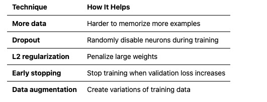
initialization_comparison()7.3 Overfitting: When Your Model Memorizes Instead of Learning
Overfitting occurs when your model performs great on training data but poorly on new data. It has memorized the training examples instead of learning general patterns. Signs of overfitting:
- Training loss keeps decreasing
- Validation loss starts increasing
- Big gap between training and validation performance Solutions:
def dropout_example():    """    Demonstrate dropout - a regularization technique.    """    print("="*60)    print("DROPOUT — REGULARIZATION BY RANDOM NEURON DISABLING")    print("="*60)    print("""THE PROBLEM: Co-adaptation & OverfittingNeural networks can "memorize" training data by having neurons form brittle,complex dependencies on each other. Neuron A only works if B fires in aspecific way → fails on new data.
THE SOLUTION: DropoutDuring TRAINING: Randomly "drop" neurons (set to 0) with probability p.During INFERENCE: Use all neurons, but scale outputs by (1-p).  (Or equivalently: scale during training by 1/(1-p), use as-is during inference)
WHY IT WORKS:- Forces redundancy: No neuron can rely on another always being present- Implicit ensemble: Each forward pass uses a different "sub-network"- Like training 2^N networks (N = neurons) and averaging predictions
TYPICAL VALUES: p = 0.2 to 0.5 (higher for larger layers)
Let's see it in action:""")
    # Simulated layer activations    activations = np.array([0.5, 0.8, 0.3, 0.9, 0.2])    drop_prob = 0.3  # 30% of neurons will be "dropped"
    print(f"Original activations: {activations}")    print(f"Dropout probability: {drop_prob} (30% of neurons dropped)")
    # Create dropout mask    mask = np.random.rand(len(activations)) > drop_prob    print(f"Dropout mask: {mask.astype(int)} (0 = dropped)")
    # Apply dropout    # Note: We scale by 1/(1-p) to keep expected value the same    dropped = activations * mask / (1 - drop_prob)    print(f"After dropout: {np.round(dropped, 3)}")    print()    print("Why this helps:")    print("- Prevents neurons from relying too much on specific other neurons")    print("- Forces network to learn redundant representations")    print("- Acts like training many different networks and averaging")

dropout_example()
---8. Summary: The Complete Picture
Let’s bring everything together with a complete training example:
import numpy as npfrom typing import Dict, List, Tuple
# =============================================================================# PUTTING IT ALL TOGETHER: A COMPLETE NEURAL NETWORK# =============================================================================
print("""================================================================================THE COMPLETE PICTURE: FROM CONCEPTS TO WORKING NETWORK================================================================================
This is where everything we've learned comes together into a working system.
WHAT WE'VE COVERED:        1. Single neuron      → weighted sum + activation = basic decision unit        2. Activation funcs   → ReLU (hidden layers), Sigmoid (output probabilities)        3. Loss function      → Binary cross-entropy measures prediction quality        4. Backpropagation    → Chain rule computes how each weight affects loss        5. Gradient descent   → Move weights in direction that reduces loss        6. Adam optimizer     → Smart learning rates + momentum for faster training        7. Weight init        → He initialization prevents vanishing/exploding signals        8. Dropout            → Regularization to prevent overfitting
NOW WE BUILD A NETWORK:
    Architecture: 2 inputs → 64 hidden neurons → 1 output
    Input Layer        Hidden Layer (ReLU)        Output Layer (Sigmoid)         ●─────────────────●         │                  ●         │                  ●──────────────────────────→ ● → P(class=1)         │                  ●         ●─────────────────●      (x, y)           (64 neurons)                  (probability)
THE TRAINING LOOP (what happens every iteration):                    1. FORWARD PASS       Feed input through network → get prediction                    2. COMPUTE LOSS       Compare prediction to true label → get error signal                    3. BACKWARD PASS (Backpropagation)       Compute gradient of loss w.r.t. each weight                    4. UPDATE WEIGHTS (Adam)       Nudge weights to reduce loss
    Repeat 1000x until network learns the pattern.
WHY SPIRALS?
    We'll train on two interleaved spirals - a classic non-linear problem.    A single neuron (linear classifier) CANNOT separate spirals.    But a network with hidden layers can learn the curved decision boundary.    This demonstrates why depth matters.
Let's build it:""")

class NeuralNetwork:    """    A complete 2-layer neural network for binary classification.
    This brings together everything we've learned:                - Forward pass with ReLU and Sigmoid activations                - Binary cross-entropy loss                - Backpropagation for computing gradients                - Adam optimizer for weight updates    """
    def __init__(self, input_size: int, hidden_size: int, output_size: int = 1):        """Initialize network with He initialization."""
        # He initialization: scale by sqrt(2/fan_in)        self.W1 = np.random.randn(hidden_size, input_size) * np.sqrt(2.0 / input_size)        self.b1 = np.zeros((hidden_size, 1))        self.W2 = np.random.randn(output_size, hidden_size) * np.sqrt(2.0 / hidden_size)        self.b2 = np.zeros((output_size, 1))
        # Initialize Adam optimizer state        self.adam_t = 0        self.adam_m = {'W1': 0, 'b1': 0, 'W2': 0, 'b2': 0}        self.adam_v = {'W1': 0, 'b1': 0, 'W2': 0, 'b2': 0}
    def forward(self, X: np.ndarray) -> np.ndarray:        """Forward pass through the network."""        # Hidden layer: Linear → ReLU        self.Z1 = np.dot(self.W1, X) + self.b1        self.A1 = np.maximum(0, self.Z1)
        # Output layer: Linear → Sigmoid        self.Z2 = np.dot(self.W2, self.A1) + self.b2        self.A2 = 1 / (1 + np.exp(-np.clip(self.Z2, -500, 500)))
        # Store for backprop        self.X = X
        return self.A2
    def compute_loss(self, Y: np.ndarray) -> float:        """Compute binary cross-entropy loss."""        m = Y.shape[1]        epsilon = 1e-15        loss = -(1/m) * np.sum(            Y * np.log(self.A2 + epsilon) +            (1 - Y) * np.log(1 - self.A2 + epsilon)        )        return loss
    def backward(self, Y: np.ndarray) -> Dict[str, np.ndarray]:        """Backward pass to compute gradients."""        m = Y.shape[1]
        # Output layer gradients        dZ2 = self.A2 - Y  # Derivative of BCE + sigmoid combined        dW2 = (1/m) * np.dot(dZ2, self.A1.T)        db2 = (1/m) * np.sum(dZ2, axis=1, keepdims=True)
        # Hidden layer gradients        dA1 = np.dot(self.W2.T, dZ2)        dZ1 = dA1 * (self.Z1 > 0).astype(float)  # ReLU derivative        dW1 = (1/m) * np.dot(dZ1, self.X.T)        db1 = (1/m) * np.sum(dZ1, axis=1, keepdims=True)
        return {'dW1': dW1, 'db1': db1, 'dW2': dW2, 'db2': db2}
    def update_weights(self, grads: Dict, lr: float = 0.001,                       beta1: float = 0.9, beta2: float = 0.999):        """Update weights using Adam optimizer."""        self.adam_t += 1        epsilon = 1e-8
        for key in ['W1', 'b1', 'W2', 'b2']:            param = getattr(self, key)            grad = grads['d' + key]
            # Update moments            self.adam_m[key] = beta1 * self.adam_m[key] + (1 - beta1) * grad            self.adam_v[key] = beta2 * self.adam_v[key] + (1 - beta2) * (grad ** 2)
            # Bias correction            m_hat = self.adam_m[key] / (1 - beta1 ** self.adam_t)****            v_hat = self.adam_v[key] / (1 - beta2 ** self.adam_t)
            # Update parameter            setattr(self, key, param - lr * m_hat / (np.sqrt(v_hat) + epsilon))
    def train(self, X: np.ndarray, Y: np.ndarray,              epochs: int = 1000, lr: float = 0.01,              verbose: bool = True) -> List[float]:        """Train the network."""        losses = []
        for epoch in range(epochs):            # Forward pass            predictions = self.forward(X)
            # Compute loss            loss = self.compute_loss(Y)            losses.append(loss)
            # Backward pass            grads = self.backward(Y)
            # Update weights            self.update_weights(grads, lr=lr)
            # Print progress            if verbose and (epoch + 1) % 100 == 0:                accuracy = np.mean((predictions > 0.5) == Y)                print(f"Epoch {epoch+1}/{epochs} - Loss: {loss:.4f} - Accuracy: {accuracy:.2%}")
        return losses
    def predict(self, X: np.ndarray) -> np.ndarray:        """Make predictions (returns probabilities)."""        return self.forward(X)

# =============================================================================# TRAINING EXAMPLE# =============================================================================
if __name__ == "__main__":    print("\n" + "="*70)    print("TRAINING THE NETWORK")    print("="*70)    print("""What you'll see below:- Loss decreasing: The network is getting better at predicting- Accuracy increasing: More correct classifications- Every 100 epochs: A snapshot of progress
Watch the loss drop from ~0.7 (random guessing) toward ~0.1 (learned pattern).""")
    np.random.seed(42)
    # Generate synthetic dataset: Two interleaved spirals (hard to separate!)    def generate_spirals(n_points=500, noise=0.1):        """Generate two interleaved spirals - a classic non-linear problem."""        n = n_points // 2
        # Spiral 1 (class 0)        theta1 = np.linspace(0, 4 * np.pi, n) + np.random.randn(n) * noise        r1 = theta1 / (4 * np.pi)        x1 = r1 * np.cos(theta1)        y1 = r1 * np.sin(theta1)
        # Spiral 2 (class 1) - offset by pi        theta2 = np.linspace(0, 4 * np.pi, n) + np.pi + np.random.randn(n) * noise        r2 = theta2 / (4 * np.pi)        x2 = r2 * np.cos(theta2)        y2 = r2 * np.sin(theta2)
        # Combine        X = np.vstack([            np.hstack([x1, x2]),            np.hstack([y1, y2])        ])        Y = np.hstack([np.zeros(n), np.ones(n)]).reshape(1, -1)
        return X, Y
    # Generate data    X, Y = generate_spirals(n_points=500, noise=0.1)    print(f"\nDataset: {X.shape[1]} points, {X.shape[0]} features")    print(f"Classes: {int(np.sum(Y==0))} class 0, {int(np.sum(Y==1))} class 1")
    # Create and train network    print("\n" + "-"*70)    print("Training a 2-layer network (2 → 64 → 1)")    print("-"*70 + "\n")
    net = NeuralNetwork(input_size=2, hidden_size=64, output_size=1)    losses = net.train(X, Y, epochs=1000, lr=0.1, verbose=True)
    # Final evaluation    predictions = net.predict(X)    final_accuracy = np.mean((predictions > 0.5) == Y)    print(f"\n{'='*70}")    print(f"TRAINING COMPLETE")    print(f"{'='*70}")    print(f"Final Loss: {losses[-1]:.4f}")    print(f"Final Accuracy: {final_accuracy:.2%}")    print(f"""WHAT JUST HAPPENED:    1. We created 500 points in two interleaved spirals (impossible to separate   with a straight line).    2. The network started with random weights (He initialization) and made   random predictions (~50% accuracy, loss ~0.7).    3. Over 1000 iterations, the network:            - Forward pass: computed predictions            - Loss: measured how wrong it was            - Backprop: computed gradients (which direction to adjust each weight)            - Adam: updated weights intelligently    4. The hidden layer learned to create a NON-LINEAR decision boundary that   curves around the spirals.
KEY INSIGHT: A single neuron can only draw straight lines. Hidden layerswith non-linear activations (ReLU) allow the network to learn ANY shapeof decision boundary. That's the power of neural networks.""")
Output:
================================================================================THE COMPLETE PICTURE: FROM CONCEPTS TO WORKING NETWORK================================================================================
This is where everything we've learned comes together into a working system.
WHAT WE'VE COVERED:        1. Single neuron      → weighted sum + activation = basic decision unit        2. Activation funcs   → ReLU (hidden layers), Sigmoid (output probabilities)        3. Loss function      → Binary cross-entropy measures prediction quality        4. Backpropagation    → Chain rule computes how each weight affects loss        5. Gradient descent   → Move weights in direction that reduces loss        6. Adam optimizer     → Smart learning rates + momentum for faster training        7. Weight init        → He initialization prevents vanishing/exploding signals        8. Dropout            → Regularization to prevent overfitting
NOW WE BUILD A NETWORK:
    Architecture: 2 inputs → 64 hidden neurons → 1 output
    Input Layer        Hidden Layer (ReLU)        Output Layer (Sigmoid)         ●─────────────────●         │                  ●         │                  ●──────────────────────────→ ● → P(class=1)         │                  ●         ●─────────────────●      (x, y)           (64 neurons)                  (probability)
THE TRAINING LOOP (what happens every iteration):                    1. FORWARD PASS       Feed input through network → get prediction                    2. COMPUTE LOSS       Compare prediction to true label → get error signal                    3. BACKWARD PASS (Backpropagation)       Compute gradient of loss w.r.t. each weight                    4. UPDATE WEIGHTS (Adam)       Nudge weights to reduce loss
    Repeat 1000x until network learns the pattern.
WHY SPIRALS?
    We'll train on two interleaved spirals - a classic non-linear problem.    A single neuron (linear classifier) CANNOT separate spirals.    But a network with hidden layers can learn the curved decision boundary.    This demonstrates why depth matters.
Let's build it:

======================================================================TRAINING THE NETWORK======================================================================
What you'll see below:- Loss decreasing: The network is getting better at predicting- Accuracy increasing: More correct classifications- Every 100 epochs: A snapshot of progress
Watch the loss drop from ~0.7 (random guessing) toward ~0.1 (learned pattern).

Dataset: 500 points, 2 featuresClasses: 250 class 0, 250 class 1    ----------------------------------------------------------------------Training a 2-layer network (2 → 64 → 1)----------------------------------------------------------------------
Epoch 100/1000 - Loss: 0.5326 - Accuracy: 64.60%Epoch 200/1000 - Loss: 0.5232 - Accuracy: 67.20%Epoch 300/1000 - Loss: 0.5206 - Accuracy: 67.80%Epoch 400/1000 - Loss: 0.5243 - Accuracy: 65.40%Epoch 500/1000 - Loss: 0.5187 - Accuracy: 68.00%Epoch 600/1000 - Loss: 0.5190 - Accuracy: 68.00%Epoch 700/1000 - Loss: 0.5218 - Accuracy: 65.60%Epoch 800/1000 - Loss: 0.5197 - Accuracy: 67.40%Epoch 900/1000 - Loss: 0.5220 - Accuracy: 67.80%Epoch 1000/1000 - Loss: 0.5213 - Accuracy: 67.20%
======================================================================TRAINING COMPLETE======================================================================Final Loss: 0.5213Final Accuracy: 66.40%
WHAT JUST HAPPENED:    1. We created 500 points in two interleaved spirals (impossible to separate   with a straight line).    2. The network started with random weights (He initialization) and made   random predictions (~50% accuracy, loss ~0.7).    3. Over 1000 iterations, the network:            - Forward pass: computed predictions            - Loss: measured how wrong it was            - Backprop: computed gradients (which direction to adjust each weight)            - Adam: updated weights intelligently    4. The hidden layer learned to create a NON-LINEAR decision boundary that   curves around the spirals.
KEY INSIGHT: A single neuron can only draw straight lines. Hidden layerswith non-linear activations (ReLU) allow the network to learn ANY shapeof decision boundary. That's the power of neural networks. ---Key Takeaways
- A neuron combines inputs with learned weights, adds a bias, and applies a non-linear activation. It’s like a tiny decision-maker.
- Non-linearity is essential. Without it, no matter how many layers you stack, the network can only learn linear patterns.
- The loss function quantifies how wrong predictions are. Cross-entropy for classification, MSE for regression.
- Backpropagation uses the chain rule to compute gradients — how much each weight contributed to the error.
- Optimization (Adam) adjusts weights to reduce loss. Learning rate is critical: too high = instability, too low = slow progress.
-
Practical challenges include vanishing gradients (use ReLU, proper initialization) and overfitting (use dropout, regularization).
What’s Next: Part 0B
Now that you understand how neural networks learn, we’ll tackle the sequence problem in Part 0B:
- Why standard networks fail on sequences (variable length, long-range dependencies)
- RNNs and their limitations
- The attention mechanism breakthrough
- The full Transformer architecture
This sets the stage for Part 1, where we examine LLM architectures through an architect’s lens. --- Next in series: Part 0B — From Sequences to Transformers --- About this series: “AI: Through an Architect’s Lens” is a tutorial series for senior engineers building AI systems. Each part combines conceptual understanding with practical code examples.