Part 0B: From Sequences to Transformers
The journey from “words in order” to “understanding meaning” — how we taught machines to process language, and why the Transformer changed everything.
AI: Through an Architect’s Lens — Part 0B
The journey from “words in order” to “understanding meaning” — how we taught machines to process language, and why the Transformer changed everything.

Target Audience: Senior engineers building foundational ML understanding
Prerequisites: Part 0A (Neural Networks & The Learning Mechanism)
Reading Time: 90–120 minutes
Series Context: Final foundation before LLM Architecture (Part 1)
Code: https://github.com/phoenixtb/ai_through_architects_lens/tree/main/0B
A Note on the Code Blocks
The code examples in this tutorial do more than demonstrate implementation — they tell stories. You’ll find ASCII diagrams, step-by-step narratives, and “why it matters” explanations embedded right in the output.
Take a moment to read through the printed output, not just the code itself. That’s where much of the intuition lives.
Companion Notebooks: This tutorial has accompanying Jupyter notebooks with runnable code and live demos. Check the GitHub repository for the full implementation.
Introduction: The Sequence Problem
In Part 0A, we learned how neural networks map inputs to outputs. We fed in features (income, credit score) and got predictions (approve/reject). But we made a crucial assumption: the inputs had a fixed size.
What happens when inputs have variable length and order matters?
Consider these sentences:
- “The bank approved the loan” (financial institution)
- “I sat by the river bank” (edge of water)
- “Bank the airplane to the left” (tilt/turn)
The word “bank” has completely different meanings depending on the words around it. To understand “bank,” you need to understand the context — the other words in the sequence and their relationships.
This is the sequence problem: How do we build neural networks that can process inputs of varying lengths where the order and relationships between elements matter?
This problem appears everywhere:
- Language: Sentences have variable length; word meaning depends on context
- Time series: Stock prices, sensor readings, user behavior sequences
- Audio: Speech is a sequence of sound waves
- Video: Frames in temporal order
- Code: Programs are sequences of tokens with complex dependencies
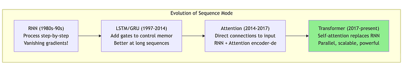
In this tutorial, we’ll trace the evolution of solutions:
- Recurrent Neural Networks (RNNs): Process sequences one step at a time
- LSTM/GRU: Remember important information longer
- Attention: Look at everything at once, focus on what matters
- Transformers: Attention is all you need
Let’s begin with understanding why standard neural networks fail on sequences.
1. Why Standard Neural Networks Fail on Sequences
1.1 The Fixed-Size Input Problem
Our loan approval network from Part 0A expected exactly 4 inputs: income, credit score, years employed, debt. What if we want to process text?
# This works - fixed 4 inputsloan_features = [45000, 680, 3, 12000]prediction = network.forward(loan_features)
# But what about text?sentence1 = ["The", "cat", "sat"]           # 3 wordssentence2 = ["The", "quick", "brown", "fox", "jumps"]  # 5 wordssentence3 = ["Hi"]                           # 1 word
# Problem: Different lengths! Our network expects fixed input size.
Naive solution 1: Pad everything to max length
max_length = 10# Pad shorter sentences with a special tokensentence1_padded = ["The", "cat", "sat", "PAD", "PAD", "PAD", "PAD", "PAD", "PAD", "PAD"]This wastes computation and doesn’t scale. What if the longest sentence is 1000 words? Every 3-word sentence would carry 997 padding tokens.
Naive solution 2: Truncate to fixed length
fixed_length = 5# Truncate longer sentenceslong_sentence = ["The", "answer", "to", "everything", "is", "clearly", "42"]truncated = long_sentence[:5] # Loses "clearly" and "42"!This loses information. In many cases, the most important words are at the end.
1.2 The Order Problem
Even if we solve the length problem, standard networks don’t understand order.
import numpy as np
# Suppose we convert words to numbers (embeddings, explained later)# and feed them to a standard network
sentence_a = [0.2, 0.8, 0.5]  # "dog bites man" → [dog, bites, man]sentence_b = [0.5, 0.8, 0.2]  # "man bites dog" → [man, bites, dog]
# A standard fully-connected layer doesn't care about order!# It just computes: W @ input + b## W @ [0.2, 0.8, 0.5] gives DIFFERENT result than W @ [0.5, 0.8, 0.2]# but only because the VALUES are in different positions,# not because the network understands that position matters.
# The network has no concept that position 0 is "subject"# and position 2 is "object"
1.3 The Long-Range Dependency Problem
Language has dependencies that span many words:
“The cat, which had been sleeping on the warm windowsill all afternoon while the rain poured outside, finally woke up.”
The verb “woke” must agree with “cat” (singular), but they’re separated by 18 words! A network needs to “remember” information across long distances.
These three problems — variable length, order sensitivity, and long-range dependencies — define the sequence modeling challenge. Let’s see how RNNs attempted to solve them.
2. Recurrent Neural Networks: Processing One Step at a Time
2.1 The Key Idea: Hidden State as Memory
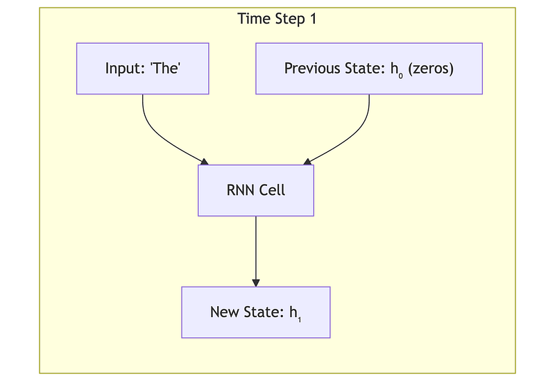
The breakthrough idea of RNNs: process the sequence one element at a time, maintaining a “memory” of what you’ve seen so far.
Imagine reading a sentence word by word:
- Read “The” → remember: “we’re starting a sentence”
- Read “cat” → remember: “the subject is a cat”
- Read “sat” → remember: “the cat is sitting”
- Read “on” → remember: “cat is sitting on something”
- Read “the” → remember: “waiting to learn what the cat sat on”
- Read “mat” → understand: “the cat sat on the mat”
At each step, you update your mental model based on the new word AND your previous understanding. This is exactly what an RNN does.


2.2 The RNN Equations
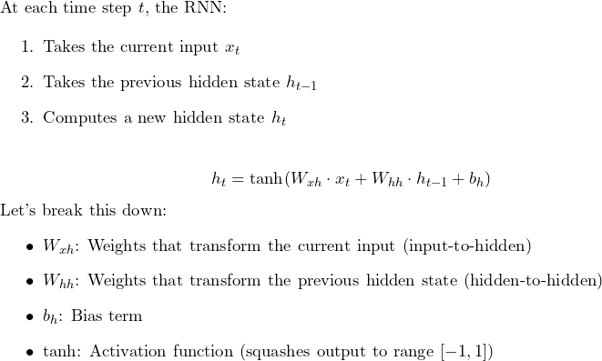
The same weights are used at every time step — this is called weight sharing and is what allows RNNs to handle variable-length sequences.
2.3 RNN Implementation
import numpy as np
class SimpleRNN:    """    A simple Recurrent Neural Network cell.
    The RNN processes sequences one element at a time, maintaining a "hidden state"    that serves as memory of what it has seen so far.
    Think of it like reading a book: as you read each word, you update your    understanding of the story. The hidden state is your "mental model" of    the story so far.
    Key insight: The SAME weights are used at every time step. This means:    1. The network can handle sequences of any length    2. What it learns about processing position 1 applies to position 100    3. The number of parameters doesn't grow with sequence length    """
    def __init__(self, input_size, hidden_size):        """        Initialize the RNN.
        Parameters        ----------        input_size : int            Dimension of each input element.            For text: This would be the word embedding dimension (e.g., 256)            For time series: This might be 1 (single value) or more (multiple sensors)
        hidden_size : int            Dimension of the hidden state (the "memory").            Larger = more capacity to remember, but more computation.            Typical values: 128, 256, 512        """        self.input_size = input_size        self.hidden_size = hidden_size
        # =====================================================================        # Weight Initialization        # =====================================================================        # We use Xavier initialization (explained in Part 0A: it keeps        # gradients stable by scaling weights based on layer sizes)
        # Weights for transforming the input        # Shape: (hidden_size, input_size)        # These weights determine how the current input affects the hidden state        scale_xh = np.sqrt(1.0 / input_size)        self.W_xh = np.random.randn(hidden_size, input_size) * scale_xh
        # Weights for transforming the previous hidden state        # Shape: (hidden_size, hidden_size)        # These weights determine how the previous memory affects the new memory        scale_hh = np.sqrt(1.0 / hidden_size)        self.W_hh = np.random.randn(hidden_size, hidden_size) * scale_hh
        # Bias for the hidden state        # Shape: (hidden_size, 1)        self.b_h = np.zeros((hidden_size, 1))
        print(f"RNN initialized:")        print(f"  Input size: {input_size}")        print(f"  Hidden size: {hidden_size}")        print(f"  W_xh shape: {self.W_xh.shape} (input → hidden)")        print(f"  W_hh shape: {self.W_hh.shape} (hidden → hidden)")        print(f"  Total parameters: {self.W_xh.size + self.W_hh.size + self.b_h.size}")
    def step(self, x_t, h_prev, verbose=False):        """        Process ONE time step of the sequence.
        This is the core RNN computation:        h_t = tanh(W_xh @ x_t + W_hh @ h_prev + b_h)
        Parameters        ----------        x_t : numpy array, shape (input_size, 1)            The input at the current time step.            For text: The word embedding of the current word.
        h_prev : numpy array, shape (hidden_size, 1)            The hidden state from the previous time step.            This encodes everything the network "remembers" so far.
        verbose : bool            If True, print intermediate computations.
        Returns        -------        h_t : numpy array, shape (hidden_size, 1)            The new hidden state after processing this input.        """
        if verbose:            print(f"\n  --- RNN Step ---")            print(f"  Input x_t shape: {x_t.shape}")            print(f"  Previous hidden h_prev shape: {h_prev.shape}")
        # Step 1: Transform the current input        # This extracts features from the current input        input_contribution = np.dot(self.W_xh, x_t)
        if verbose:            print(f"  W_xh @ x_t: shape {input_contribution.shape}")
        # Step 2: Transform the previous hidden state        # This carries forward the memory from previous steps        memory_contribution = np.dot(self.W_hh, h_prev)
        if verbose:            print(f"  W_hh @ h_prev: shape {memory_contribution.shape}")
        # Step 3: Combine and add bias        # The new hidden state is influenced by BOTH current input AND memory        combined = input_contribution + memory_contribution + self.b_h
        # Step 4: Apply tanh activation        # tanh squashes values to [-1, 1], which helps with:        # - Keeping hidden state bounded (doesn't explode)        # - Introducing non-linearity (can learn complex patterns)        h_t = np.tanh(combined)
        if verbose:            print(f"  New hidden state h_t: shape {h_t.shape}")            print(f"  Hidden state range: [{h_t.min():.3f}, {h_t.max():.3f}]")
        return h_t
    def forward(self, X, verbose=False):        """        Process an entire sequence.
        Parameters        ----------        X : numpy array, shape (sequence_length, input_size)            The full input sequence.            Each row is one time step.
        verbose : bool            If True, print step-by-step details.
        Returns        -------        hidden_states : list of numpy arrays            The hidden state after each time step.            hidden_states[-1] is the final "summary" of the entire sequence.        """        sequence_length = X.shape[0]
        # Initialize hidden state to zeros        # This represents "no memory yet" at the start        h = np.zeros((self.hidden_size, 1))
        hidden_states = []
        if verbose:            print(f"\nProcessing sequence of length {sequence_length}")            print("=" * 50)
        for t in range(sequence_length):            # Get input at time t            # Reshape to (input_size, 1) for matrix multiplication            x_t = X[t:t+1, :].T
            if verbose:                print(f"\nTime step {t}:")
            # Process this time step            h = self.step(x_t, h, verbose=verbose)
            # Store the hidden state            hidden_states.append(h.copy())
        if verbose:            print("\n" + "=" * 50)            print(f"Sequence processing complete!")            print(f"Final hidden state encodes the entire sequence.")
        return hidden_states

# =============================================================================# DEMONSTRATION# =============================================================================
print("=" * 70)print("RECURRENT NEURAL NETWORKS (RNNs)")print("=" * 70)print("""THE PROBLEM: Standard neural networks expect FIXED-SIZE inputs.But sequences (text, audio, time series) have VARIABLE length and ORDER matters.
"dog bites man" ≠ "man bites dog"  (same words, different meaning!)
THE SOLUTION: Process one element at a time, maintaining a "hidden state"that acts as MEMORY of what we've seen so far.
At each time step t:  h_t = tanh(W_xh @ x_t + W_hh @ h_prev + b)
  - x_t: current input (e.g., word embedding)  - h_prev: memory from previous steps  - h_t: updated memory after seeing this input
KEY INSIGHT: Same weights (W_xh, W_hh) are used at EVERY time step.This means:  1. Network can handle ANY sequence length  2. What it learns at position 1 applies to position 100  3. Parameters don't grow with sequence length
Let's see it in action:""")
# Create a simple RNNrnn = SimpleRNN(input_size=4, hidden_size=3)
# Create a dummy sequence (3 time steps, 4 features each)# In practice, these would be word embeddings or sensor readingssequence = np.array([    [0.1, 0.2, 0.3, 0.4],  # Time step 0    [0.5, 0.6, 0.7, 0.8],  # Time step 1    [0.2, 0.1, 0.4, 0.3],  # Time step 2])
print(f"\nInput sequence shape: {sequence.shape}")print(f"(3 time steps, 4 features per step)")
# Process the sequencehidden_states = rnn.forward(sequence, verbose=True)
print(f"\nNumber of hidden states: {len(hidden_states)}")print(f"Final hidden state (summary of entire sequence):")print(hidden_states[-1].flatten())
print("""KEY TAKEAWAY:The final hidden state h_3 is a fixed-size vector that "summarizes" theentire input sequence. This can be used for:  - Sentiment analysis: sequence → h_final → positive/negative  - Language modeling: at each step, h_t → predict next word  - Seq2Seq: encode input → h_final → decode to output
LIMITATION (covered next): Gradients vanish over long sequences.After ~10-20 steps, early inputs barely affect learning.This is why LSTM/GRU were invented.""")
2.4 What the Hidden State Captures


The same RNN architecture can be used for different tasks:
Sentiment Analysis (many-to-one): Read all words → final hidden state → positive/negative
Language Modeling (many-to-many): At each step, predict the next word
Sequence-to-Sequence (encoder-decoder): Encode input sequence → decode to output sequence
2.5 The Problem: Vanishing Gradients Strike Again
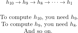
RNNs have a fundamental flaw. Remember from Part 0A how gradients can vanish when multiplied through many layers? In RNNs, the problem is worse because we multiply through many time steps.
When training an RNN with backpropagation, gradients flow backward through time.

The tanh derivative is at most 1.0, and typically much smaller. After multiplying many small numbers, the gradient vanishes:
def demonstrate_rnn_vanishing_gradient():    """    Show why gradients vanish in RNNs over long sequences.    """    print("=" * 70)    print("THE VANISHING GRADIENT PROBLEM IN RNNs")    print("=" * 70)    print("""WHY THIS MATTERS:
Consider: "The cat, which had been sleeping on the warm windowsillall afternoon while the rain poured outside, finally woke up."
The verb "woke" must agree with "cat" (singular) — but they're 18 words apart!For the RNN to learn this, the gradient from "woke" must flow back to "cat".
THE PROBLEM:
During backpropagation, gradients flow backward through time.At each step, we multiply by:  - The derivative of tanh (max 1.0, typically ~0.5)  - The weight matrix W_hh (typically < 1.0 to avoid explosion)
After N steps: gradient ≈ (0.5 × 0.9)^N = 0.45^N
Let's see what happens:""")
    # tanh derivative: max value is 1.0 (at tanh(0) = 0)    # For typical values, it's much smaller    # d/dx tanh(x) = 1 - tanh(x)²
    # Simulate gradient flow through time    # Each time step multiplies gradient by tanh_derivative and W_hh
    # Assume typical tanh derivative of ~0.5 and well-initialized W_hh    tanh_deriv_typical = 0.5    w_hh_effect = 0.9  # Slightly less than 1
    gradient_multiplier_per_step = tanh_deriv_typical * w_hh_effect
    print(f"Gradient multiplier per time step: {gradient_multiplier_per_step}")    print()
    gradient = 1.0  # Start with gradient = 1 from the loss
    for t in [1, 5, 10, 20, 50, 100]:        gradient_at_t = gradient_multiplier_per_step ** t        print(f"After {t:3d} time steps: gradient magnitude = {gradient_at_t:.2e}")
    print()    print("After 100 steps, gradient is essentially ZERO!")    print("Early words in a long sequence barely get any learning signal.")    print()    print("""This is catastrophic for language understanding. In our example sentence,the RNN can't connect "cat" to "woke" because the gradient vanishesover those 18 words.
THE SOLUTION: LSTM (Long Short-Term Memory)
LSTM introduces a "cell state" — a highway for information that usesADDITION instead of multiplication. Gradients can flow through additionwithout vanishing. Plus, learnable "gates" control what to remember/forget.
That's what we'll build next.""")

demonstrate_rnn_vanishing_gradient()
Output:
======================================================================THE VANISHING GRADIENT PROBLEM IN RNNs======================================================================
WHY THIS MATTERS:
Consider: "The cat, which had been sleeping on the warm windowsillall afternoon while the rain poured outside, finally woke up."
The verb "woke" must agree with "cat" (singular) — but they're 18 words apart!For the RNN to learn this, the gradient from "woke" must flow back to "cat".
THE PROBLEM:
During backpropagation, gradients flow backward through time.At each step, we multiply by:  - The derivative of tanh (max 1.0, typically ~0.5)  - The weight matrix W_hh (typically < 1.0 to avoid explosion)
After N steps: gradient ≈ (0.5 × 0.9)^N = 0.45^N
Let's see what happens:
Gradient multiplier per time step: 0.45
After   1 time steps: gradient magnitude = 4.50e-01After   5 time steps: gradient magnitude = 1.85e-02After  10 time steps: gradient magnitude = 3.41e-04After  20 time steps: gradient magnitude = 1.16e-07After  50 time steps: gradient magnitude = 4.58e-18After 100 time steps: gradient magnitude = 2.10e-35
After 100 steps, gradient is essentially ZERO!Early words in a long sequence barely get any learning signal.
This is catastrophic for language understanding. In our example sentence,the RNN can't connect "cat" to "woke" because the gradient vanishesover those 18 words.
THE SOLUTION: LSTM (Long Short-Term Memory)
LSTM introduces a "cell state" — a highway for information that usesADDITION instead of multiplication. Gradients can flow through additionwithout vanishing. Plus, learnable "gates" control what to remember/forget.
That's what we'll build next.
This is catastrophic for language understanding. In the sentence “The cat, which had been sleeping on the warm windowsill all afternoon while the rain poured outside, finally woke up,” the RNN can’t connect “cat” to “woke” because the gradient vanishes over those 18 words.
3. LSTM: Learning to Remember
3.1 The Key Innovation: Gating Mechanisms
In 1997, Hochreiter and Schmidhuber introduced Long Short-Term Memory (LSTM) networks. The key insight: let the network learn what to remember and what to forget.
Standard RNN: “Here’s new input. Let me mix it with my memory somehow.”
LSTM: “Here’s new input. Should I:
- Forget some of my old memory?
- Add this new information to my memory?
- Output some of my memory right now?”
These decisions are made by gates — neural networks that output values between 0 (completely block) and 1 (completely allow).
3.2 The Three Gates
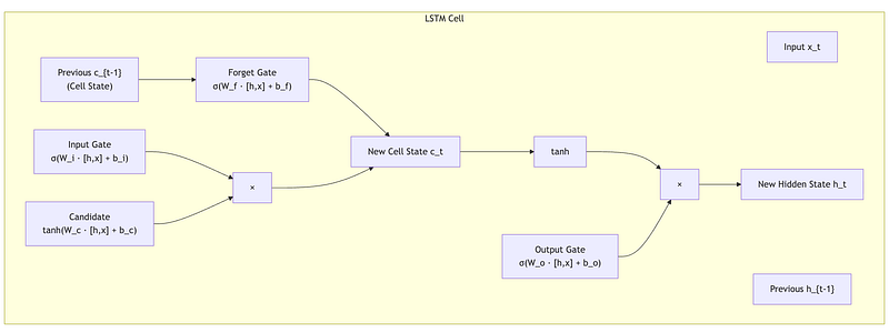
Gate 1: Forget Gate (What should I forget?)

The forget gate looks at the previous hidden state and current input, and outputs a number between 0 and 1 for each element of the cell state. A value of 0 means “completely forget this,” and 1 means “completely keep this.”
Example: When processing “She finished her project. He started…”, the forget gate might forget the “she” context when it sees “He.”
Gate 2: Input Gate (What new information should I store?)

Example: When processing “The capital of France is Paris,” the input gate should strongly store “Paris” as the answer.
Gate 3: Output Gate (What should I output?

Example: If the cell state stores both “subject is cat” and “verb is past tense,” the output gate might only expose the subject when generating the next word prediction.
3.3 The Cell State: The Memory Highway

This is just: (forget some old stuff) + (add some new stuff).
Crucially, this is mostly addition, not multiplication! Gradients can flow through the cell state without repeated multiplication, avoiding the vanishing gradient problem.
Think of it like a conveyor belt. Information can ride along, with gates occasionally adding or removing things. This is much better than the RNN approach where everything gets mixed together at every step.
3.4 LSTM Implementation
import numpy as np
class LSTM:    """    Long Short-Term Memory network.
    LSTM solves the vanishing gradient problem of standard RNNs by introducing:    1. A separate "cell state" that carries information across time steps    2. Gates that control what information flows in and out
    The key insight: Instead of always mixing old and new information,    let the network LEARN when to remember and when to forget.
    Think of it like a notepad:    - Forget gate: Eraser (which notes to erase?)    - Input gate: Pen (which new notes to write?)    - Output gate: Highlighter (which notes are relevant right now?)    - Cell state: The notepad itself (persistent storage)    """
    def __init__(self, input_size, hidden_size):        """        Initialize LSTM.
        Parameters        ----------        input_size : int            Dimension of each input element (e.g., word embedding size)        hidden_size : int            Dimension of hidden state and cell state        """        self.input_size = input_size        self.hidden_size = hidden_size
        # Combined input: [h_{t-1}, x_t] has size (hidden_size + input_size)        combined_size = hidden_size + input_size
        # Xavier initialization scale        scale = np.sqrt(1.0 / combined_size)
        # =====================================================================        # Forget Gate: Decides what to erase from cell state        # =====================================================================        # Output is between 0 (forget completely) and 1 (keep completely)        self.W_f = np.random.randn(hidden_size, combined_size) * scale        self.b_f = np.zeros((hidden_size, 1))
        # =====================================================================        # Input Gate: Decides what new information to store        # =====================================================================        self.W_i = np.random.randn(hidden_size, combined_size) * scale        self.b_i = np.zeros((hidden_size, 1))
        # =====================================================================        # Candidate Values: The new information that COULD be stored        # =====================================================================        self.W_c = np.random.randn(hidden_size, combined_size) * scale        self.b_c = np.zeros((hidden_size, 1))
        # =====================================================================        # Output Gate: Decides what to output from cell state        # =====================================================================        self.W_o = np.random.randn(hidden_size, combined_size) * scale        self.b_o = np.zeros((hidden_size, 1))
        total_params = 4 * (self.W_f.size + self.b_f.size)        print(f"LSTM initialized:")        print(f"  Input size: {input_size}")        print(f"  Hidden size: {hidden_size}")        print(f"  Total parameters: {total_params}")        print(f"  (Note: 4x more parameters than simple RNN due to 4 gates)")
    def sigmoid(self, x):        """Sigmoid activation: squashes to (0, 1) for gating."""        return 1 / (1 + np.exp(-np.clip(x, -500, 500)))
    def step(self, x_t, h_prev, c_prev, verbose=False):        """        Process ONE time step.
        Parameters        ----------        x_t : numpy array, shape (input_size, 1)            Current input        h_prev : numpy array, shape (hidden_size, 1)            Previous hidden state (what we output last time)        c_prev : numpy array, shape (hidden_size, 1)            Previous cell state (our persistent memory)        verbose : bool            Print detailed gate activations
        Returns        -------        h_t : numpy array, shape (hidden_size, 1)            New hidden state (output)        c_t : numpy array, shape (hidden_size, 1)            New cell state (updated memory)        """
        # Concatenate previous hidden state and current input        # This combined vector is what all gates look at        combined = np.vstack([h_prev, x_t])
        # =====================================================================        # Step 1: Forget Gate - What to erase from memory?        # =====================================================================        f_t = self.sigmoid(np.dot(self.W_f, combined) + self.b_f)        # f_t is between 0 and 1 for each cell state dimension        # 0 = completely forget, 1 = completely keep
        if verbose:            print(f"  Forget gate (avg): {f_t.mean():.3f} (0=forget all, 1=keep all)")
        # =====================================================================        # Step 2: Input Gate - What new info to store?        # =====================================================================        i_t = self.sigmoid(np.dot(self.W_i, combined) + self.b_i)        # i_t is between 0 and 1: how much to add
        if verbose:            print(f"  Input gate (avg): {i_t.mean():.3f} (0=ignore, 1=store)")
        # =====================================================================        # Step 3: Candidate Values - The new info that COULD be stored        # =====================================================================        c_tilde = np.tanh(np.dot(self.W_c, combined) + self.b_c)        # c_tilde is between -1 and 1: the candidate new values
        if verbose:            print(f"  Candidate values range: [{c_tilde.min():.3f}, {c_tilde.max():.3f}]")
        # =====================================================================        # Step 4: Update Cell State - The actual memory update        # =====================================================================        # This is the key equation! Mostly addition, not multiplication.        # c_t = (forget some old) + (add some new)        c_t = f_t * c_prev + i_t * c_tilde
        if verbose:            print(f"  Cell state updated: range [{c_t.min():.3f}, {c_t.max():.3f}]")
        # =====================================================================        # Step 5: Output Gate - What to output?        # =====================================================================        o_t = self.sigmoid(np.dot(self.W_o, combined) + self.b_o)
        if verbose:            print(f"  Output gate (avg): {o_t.mean():.3f} (0=hide, 1=expose)")
        # =====================================================================        # Step 6: Compute Hidden State (Output)        # =====================================================================        # The hidden state is a filtered version of the cell state        h_t = o_t * np.tanh(c_t)
        if verbose:            print(f"  Hidden state range: [{h_t.min():.3f}, {h_t.max():.3f}]")
        return h_t, c_t
    def forward(self, X, verbose=False):        """        Process an entire sequence.
        Parameters        ----------        X : numpy array, shape (sequence_length, input_size)            The full input sequence
        Returns        -------        hidden_states : list            Hidden state after each time step        cell_states : list            Cell state after each time step        """        sequence_length = X.shape[0]
        # Initialize both hidden state and cell state to zeros        h = np.zeros((self.hidden_size, 1))        c = np.zeros((self.hidden_size, 1))
        hidden_states = []        cell_states = []
        if verbose:            print(f"\nProcessing sequence of length {sequence_length}")            print("=" * 60)
        for t in range(sequence_length):            x_t = X[t:t+1, :].T
            if verbose:                print(f"\nTime step {t}:")
            h, c = self.step(x_t, h, c, verbose=verbose)
            hidden_states.append(h.copy())            cell_states.append(c.copy())
        return hidden_states, cell_states

# =============================================================================# DEMONSTRATION: LSTM vs RNN on long sequences# =============================================================================
print("=" * 70)print("LSTM DEMONSTRATION")print("=" * 70)
lstm = LSTM(input_size=4, hidden_size=3)
# Create a longer sequencesequence = np.random.randn(10, 4) * 0.5  # 10 time steps
print(f"\nInput sequence shape: {sequence.shape}")print(f"(10 time steps, 4 features per step)")
hidden_states, cell_states = lstm.forward(sequence, verbose=True)
print("\n" + "=" * 70)print("KEY INSIGHT: The cell state can carry information across many steps")print("because it uses addition, not multiplication!")print("=" * 70)
3.5 GRU: A Simpler Alternative
Gated Recurrent Unit (GRU) is a simplified version of LSTM with only two gates:
- Update gate: Combines forget and input gates
- Reset gate: Controls how much past information to forget
GRU has fewer parameters than LSTM and often performs similarly. The choice between them is often empirical — try both and see which works better for your task.
# GRU equations (for reference):# z_t = σ(W_z · [h_{t-1}, x_t]) # Update gate# r_t = σ(W_r · [h_{t-1}, x_t]) # Reset gate# h̃_t = tanh(W_h · [r_t * h_{t-1}, x_t]) # Candidate# h_t = (1 - z_t) * h_{t-1} + z_t * h̃_t # New hidden state3.6 The Remaining Problem: Sequential Processing
LSTM and GRU solve the vanishing gradient problem, but they share a fundamental limitation with basic RNNs: sequential processing.
This means:
- No parallelization: Can’t process time steps in parallel on GPUs
- Long-range still hard: Even with LSTM, very long sequences (500+ tokens) are challenging
- Slow training: Must wait for sequential computation
What if we could look at the entire sequence at once?
4. Attention: Looking at Everything at Once
4.1 The Key Insight: Direct Connections
The fundamental problem with RNNs (including LSTM): information must flow step by step. To connect word 1 to word 100, information passes through 99 intermediate steps.
Attention flips this: Instead of sequential processing, create direct connections between any two positions.
Imagine you’re translating “The cat sat on the mat” to French. When generating the French word for “mat,” wouldn’t it be helpful to look directly at “mat” in the English sentence, rather than hoping that information survived 5 RNN steps?
This is attention: at each step, look at all inputs and focus on what’s relevant.
4.2 Attention in Sequence-to-Sequence Models
Attention was first introduced for machine translation (Bahdanau et al., 2014). The setup:
Encoder: Process input sentence (English) with an RNN, producing hidden states h₁, h₂ …
Decoder: Generate output sentence (French) word by word
Attention: At each decoder step, compute which encoder states are relevant

When generating “Le” (French for “The”), the model pays most attention to “The” (α₁ = 0.7).
4.3 Computing Attention Scores
How do we decide how much attention to pay to each position? We compute a score for each input position, then normalize with softmax.

The scores tell us: “How relevant is encoder position j to what I’m currently generating?”
Then we normalize to get attention weights:

This context vector cᵢ is a “summary” of the input, weighted by relevance to the current decoding step.
4.4 Attention Implementation
import numpy as np
def compute_attention(encoder_states, decoder_state, verbose=False):    """    Compute attention over encoder states given current decoder state.
    This implements "additive attention" (Bahdanau attention):    - Score each encoder state based on its relevance to the decoder state    - Normalize scores with softmax to get attention weights    - Compute weighted sum of encoder states
    Parameters    ----------    encoder_states : numpy array, shape (seq_len, hidden_size)        Hidden states from the encoder, one per input position.        Each row represents what the encoder "understood" at that position.
    decoder_state : numpy array, shape (hidden_size,)        Current decoder hidden state.        This represents "what we're trying to generate right now."
    verbose : bool        If True, print step-by-step computation.
    Returns    -------    context : numpy array, shape (hidden_size,)        Weighted sum of encoder states (the "attended" representation)    attention_weights : numpy array, shape (seq_len,)        How much attention is paid to each encoder position (sums to 1)    """    seq_len, hidden_size = encoder_states.shape
    if verbose:        print("Computing Attention")        print("=" * 60)        print(f"Encoder states: {seq_len} positions, each of size {hidden_size}")        print(f"Decoder state: size {hidden_size}")
    # =========================================================================    # Step 1: Compute attention scores    # =========================================================================    # For each encoder position, compute: "How relevant is this to the decoder?"    #    # Simple approach: dot product between encoder and decoder states    # Higher dot product = more similar = more relevant
    scores = []
    for j in range(seq_len):        # Dot product measures similarity        score = np.dot(encoder_states[j], decoder_state)        scores.append(score)
    scores = np.array(scores)
    if verbose:        print(f"\nStep 1: Raw attention scores (dot products)")        for j, score in enumerate(scores):            print(f"  Position {j}: score = {score:.4f}")
    # =========================================================================    # Step 2: Normalize with softmax    # =========================================================================    # Convert scores to probabilities that sum to 1    # Higher score → higher probability → more attention
    # Softmax with numerical stability (subtract max)    exp_scores = np.exp(scores - np.max(scores))    attention_weights = exp_scores / np.sum(exp_scores)
    if verbose:        print(f"\nStep 2: Attention weights (softmax of scores)")        for j, weight in enumerate(attention_weights):            bar = "█" * int(weight * 40)  # Visual bar            print(f"  Position {j}: {weight:.4f} {bar}")        print(f"  Sum of weights: {np.sum(attention_weights):.4f} (should be 1.0)")
    # =========================================================================    # Step 3: Compute weighted sum (context vector)    # =========================================================================    # The context vector is a weighted combination of all encoder states    # Positions with higher attention contribute more
    context = np.zeros(hidden_size)
    for j in range(seq_len):        # Each encoder state contributes proportionally to its attention weight        context += attention_weights[j] * encoder_states[j]
    if verbose:        print(f"\nStep 3: Context vector (weighted sum)")        print(f"  context = Σ(attention_weight[j] × encoder_state[j])")        print(f"  Context shape: {context.shape}")        print(f"  Context values: {context}")
    return context, attention_weights

# =============================================================================# DEMONSTRATION# =============================================================================
print("=" * 70)print("ATTENTION MECHANISM DEMONSTRATION")print("=" * 70)
np.random.seed(42)
# Simulate encoder states for a 5-word sentence# In practice, these come from an RNN or transformer encoderseq_len = 5hidden_size = 4
# Create encoder states (pretend these encode: "The cat sat on mat")encoder_states = np.array([    [0.8, 0.1, 0.1, 0.0],   # "The" - article, low information    [0.1, 0.9, 0.1, 0.1],   # "cat" - subject, high information    [0.1, 0.1, 0.8, 0.1],   # "sat" - verb    [0.3, 0.1, 0.1, 0.1],   # "on" - preposition    [0.1, 0.1, 0.2, 0.9],   # "mat" - object])
# Simulate decoder state when generating a word related to "cat"# (we want the model to pay attention to "cat")decoder_state = np.array([0.2, 0.85, 0.1, 0.1])  # Similar to "cat" encoding
print("\nScenario: Translating to French, currently generating word related to 'cat'")print("We expect attention to focus on position 1 ('cat')")
context, attention = compute_attention(encoder_states, decoder_state, verbose=True)
print("\n" + "=" * 70)print("INTERPRETATION")print("=" * 70)print(f"The model paid most attention to position 1 ('{['The', 'cat', 'sat', 'on', 'mat'][np.argmax(attention)]}')")print(f"This context vector can now be used to help generate the French word")
4.5 Why Attention Helps
Attention provides three key benefits:
Direct connections: Every output position can directly access every input position. No more vanishing gradients over long distances!
Interpretability: Attention weights show us what the model is “looking at.” This is valuable for debugging and understanding model behavior.
Parallelization (partial): While the decoder still processes sequentially, attention computation over encoder states can be parallelized.
But we still have one problem: the decoder processes one step at a time. What if we could use attention for the ENTIRE computation, with no recurrence at all?
5. Self-Attention: Attending to Yourself
5.1 The Breakthrough Idea
What if, instead of computing attention between encoder and decoder, we compute attention within a single sequence?
Consider the sentence: “The animal didn’t cross the street because it was too tired.”
What does “it” refer to? “Animal” or “street”?
To understand “it,” we need to look at other words in the same sentence and figure out relationships. This is self-attention.

“It” pays strong attention to “animal” (and also to “tired,” which provides context that it’s something that can be tired, not a street).
5.2 Query, Key, Value: The QKV Framework
Self-attention uses three concepts from information retrieval:
Query (Q): What am I looking for? Key (K): What do I contain? Value (V): What do I actually provide?
Analogy: Searching a library
- Query: “I want books about cats”
- Key: Each book’s subject tags (“cats,” “dogs,” “history”)
- Value: The actual content of the book
The attention score between positions and is computed as:
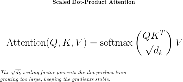
Let’s break this down step by step.
5.3 Self-Attention Step by Step
import numpy as np
def self_attention_step_by_step(X, verbose=True):    """    Demonstrate self-attention with detailed explanation.
    Self-attention allows each position in a sequence to "look at" all other    positions and compute a weighted combination based on relevance.
    The key innovation: Instead of using the same representation for everything,    we project into three different spaces:    - Query (Q): "What am I looking for?"    - Key (K): "What do I contain?"    - Value (V): "What should I contribute?"
    Parameters    ----------    X : numpy array, shape (seq_len, d_model)        Input sequence. Each row is one position's embedding.        In transformers, d_model is typically 512 or 768.
    verbose : bool        If True, print step-by-step details.
    Returns    -------    output : numpy array, shape (seq_len, d_model)        Output sequence after self-attention.        Each position now contains information gathered from all positions.    attention_weights : numpy array, shape (seq_len, seq_len)        Attention weight matrix showing how much each position attends to others.    """
    seq_len, d_model = X.shape
    if verbose:        print("=" * 70)        print("SELF-ATTENTION STEP BY STEP")        print("=" * 70)        print(f"\nInput: {seq_len} positions, each with {d_model} dimensions")
    # =========================================================================    # Step 1: Create learnable projection matrices    # =========================================================================    # In practice, these are learned during training.    # Here we'll use random matrices for demonstration.
    # d_k is the dimension of queries and keys (often d_model or d_model/num_heads)    d_k = d_model    d_v = d_model
    # W_Q projects input to query space    # W_K projects input to key space    # W_V projects input to value space    np.random.seed(42)    W_Q = np.random.randn(d_model, d_k) * 0.1    W_K = np.random.randn(d_model, d_k) * 0.1    W_V = np.random.randn(d_model, d_v) * 0.1
    if verbose:        print(f"\nStep 1: Projection matrices")        print(f"  W_Q shape: {W_Q.shape} (projects to Query space)")        print(f"  W_K shape: {W_K.shape} (projects to Key space)")        print(f"  W_V shape: {W_V.shape} (projects to Value space)")
    # =========================================================================    # Step 2: Compute Q, K, V for each position    # =========================================================================    # Each position gets its own Query, Key, and Value vector
    Q = np.dot(X, W_Q)  # Shape: (seq_len, d_k)    K = np.dot(X, W_K)  # Shape: (seq_len, d_k)    V = np.dot(X, W_V)  # Shape: (seq_len, d_v)
    if verbose:        print(f"\nStep 2: Compute Q, K, V for each position")        print(f"  Q = X @ W_Q, shape: {Q.shape}")        print(f"  K = X @ W_K, shape: {K.shape}")        print(f"  V = X @ W_V, shape: {V.shape}")        print(f"\n  Interpretation:")        print(f"  - Q[i] = What is position {0} looking for?")        print(f"  - K[i] = What does position {0} contain?")        print(f"  - V[i] = What should position {0} contribute?")
    # =========================================================================    # Step 3: Compute attention scores    # =========================================================================    # For each pair of positions (i, j):    # score[i,j] = Q[i] · K[j] = "How relevant is position j to position i?"
    # Matrix multiplication: Q @ K^T gives all pairwise dot products at once!    # Shape: (seq_len, d_k) @ (d_k, seq_len) = (seq_len, seq_len)    scores = np.dot(Q, K.T)
    if verbose:        print(f"\nStep 3: Compute attention scores (Q @ K^T)")        print(f"  Scores shape: {scores.shape}")        print(f"  scores[i,j] = How much should position i attend to position j?")        print(f"\n  Raw scores matrix:")        for i in range(seq_len):            row = " ".join([f"{s:6.2f}" for s in scores[i]])            print(f"    Position {i}: [{row}]")
    # =========================================================================    # Step 4: Scale by sqrt(d_k)    # =========================================================================    # Why scale? Dot products grow with dimension size.    # Large values → softmax outputs very peaked (all weight on one position)    # Scaling keeps the variance manageable.
    scale = np.sqrt(d_k)    scaled_scores = scores / scale
    if verbose:        print(f"\nStep 4: Scale by √d_k = √{d_k} = {scale:.2f}")        print(f"  Why? Large dot products make softmax too 'peaky'")        print(f"  Scaled scores range: [{scaled_scores.min():.2f}, {scaled_scores.max():.2f}]")
    # =========================================================================    # Step 5: Apply softmax (row-wise)    # =========================================================================    # Convert scores to probabilities    # Each row sums to 1: attention_weights[i] sums to 1
    def softmax(x, axis=-1):        exp_x = np.exp(x - np.max(x, axis=axis, keepdims=True))        return exp_x / np.sum(exp_x, axis=axis, keepdims=True)
    attention_weights = softmax(scaled_scores, axis=1)
    if verbose:        print(f"\nStep 5: Apply softmax (convert to probabilities)")        print(f"  Each row now sums to 1.0")        print(f"\n  Attention weight matrix:")        for i in range(seq_len):            row = " ".join([f"{w:5.3f}" for w in attention_weights[i]])            max_j = np.argmax(attention_weights[i])            print(f"    Position {i}: [{row}] → focuses on position {max_j}")
    # =========================================================================    # Step 6: Compute weighted sum of values    # =========================================================================    # For each position i:    # output[i] = sum over j of (attention_weight[i,j] * V[j])    #    # Matrix form: attention_weights @ V    # Shape: (seq_len, seq_len) @ (seq_len, d_v) = (seq_len, d_v)
    output = np.dot(attention_weights, V)
    if verbose:        print(f"\nStep 6: Compute weighted sum of values")        print(f"  output = attention_weights @ V")        print(f"  Output shape: {output.shape}")        print(f"\n  Interpretation:")        print(f"  output[i] now contains information from ALL positions,")        print(f"  weighted by how relevant each position is to position i.")
    return output, attention_weights

# =============================================================================# DEMONSTRATION# =============================================================================
# Create a simple sequence (3 positions, 4 dimensions each)# Pretend this represents: ["The", "cat", "sat"]# with each word having a 4-dimensional embedding
X = np.array([    [1.0, 0.0, 0.0, 0.0],   # "The" - article    [0.0, 1.0, 0.5, 0.0],   # "cat" - noun, animate    [0.0, 0.0, 0.0, 1.0],   # "sat" - verb])
output, attention_weights = self_attention_step_by_step(X, verbose=True)
print("\n" + "=" * 70)print("KEY INSIGHT")print("=" * 70)print("""After self-attention, each position's representation incorporatesinformation from ALL other positions, weighted by relevance.
This is different from RNNs:- RNN: Position 3 only "sees" position 1 through position 2- Self-attention: Position 3 directly attends to position 1
This direct connection is why transformers handle long-rangedependencies so much better than RNNs!""")
5.4 Why Self-Attention is Revolutionary
Parallelization: All attention scores can be computed in parallel. No sequential dependency like RNNs.
Constant path length: Every position is directly connected to every other position. Information doesn’t degrade over distance.
Flexibility: Attention weights are computed dynamically based on content. The same word can attend to different things in different contexts.
6. The Transformer: Putting It All Together
6.1 “Attention Is All You Need”
In 2017, Vaswani et al. published a paper with this provocative title. Their key claim: we don’t need RNNs or convolutions. Self-attention alone can handle sequence processing.
The result was the Transformer architecture, which powers GPT, BERT, T5, and virtually all modern LLMs.
6.2 The Transformer Architecture
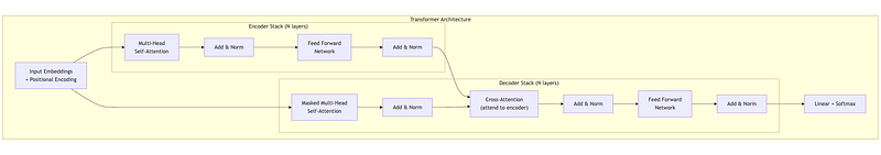
Let’s understand each component.
6.3 Component 1: Input Embeddings
Words are discrete tokens. We need to convert them to continuous vectors for the neural network.
Word Embeddings: Each word is mapped to a learned vector. Words with similar meanings have similar vectors.
# Conceptual example (real embeddings are learned)embeddings = { "cat": [0.2, 0.8, 0.1, ...], # 512 or 768 dimensions "dog": [0.25, 0.75, 0.15, ...], # Similar to cat! "the": [0.9, 0.1, 0.05, ...], # Different from cat/dog}Positional Encoding: Self-attention has no inherent notion of position. We must explicitly inject position information.
The original Transformer uses sinusoidal positional encoding:

def positional_encoding(max_seq_len, d_model):    """    Compute sinusoidal positional encoding.
    Why sinusoidal?    1. Deterministic (no learning required)    2. Can extrapolate to longer sequences than seen in training    3. Relative positions can be computed via linear transformation
    Parameters    ----------    max_seq_len : int        Maximum sequence length to generate encodings for    d_model : int        Dimension of the model (embedding dimension)
    Returns    -------    PE : numpy array, shape (max_seq_len, d_model)        Positional encodings. Add these to word embeddings.    """
    # Create position indices: [0, 1, 2, ..., max_seq_len-1]    positions = np.arange(max_seq_len)[:, np.newaxis]  # Shape: (max_seq_len, 1)
    # Create dimension indices: [0, 1, 2, ..., d_model-1]    dims = np.arange(d_model)[np.newaxis, :]  # Shape: (1, d_model)
    # Compute the angles    # The division by 10000^(2i/d_model) creates different frequencies    # for different dimensions    angles = positions / np.power(10000, (2 * (dims // 2)) / d_model)
    # Apply sin to even indices, cos to odd indices    PE = np.zeros((max_seq_len, d_model))    PE[:, 0::2] = np.sin(angles[:, 0::2])  # Even dimensions: sin    PE[:, 1::2] = np.cos(angles[:, 1::2])  # Odd dimensions: cos
    return PE

# Visualize positional encodingPE = positional_encoding(max_seq_len=50, d_model=64)
print("Positional Encoding Visualization")print("=" * 60)print(f"Shape: {PE.shape} (50 positions, 64 dimensions)")print(f"\nEach position gets a unique pattern of sin/cos values.")print(f"These are ADDED to word embeddings to inject position info.")print(f"\nPosition 0, first 8 dims: {PE[0, :8].round(3)}")print(f"Position 1, first 8 dims: {PE[1, :8].round(3)}")print(f"Position 2, first 8 dims: {PE[2, :8].round(3)}")
6.4 Component 2: Multi-Head Attention
Instead of computing attention once, we compute it multiple times with different learned projections. This allows the model to capture different types of relationships.
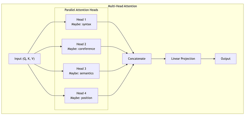
Each head might learn to focus on different things:
- Head 1: Subject-verb agreement
- Head 2: Pronoun resolution (what does “it” refer to?)
- Head 3: Semantic similarity
- Head 4: Nearby words
print("=" * 70)print("MULTI-HEAD ATTENTION")print("=" * 70)print("""WHY MULTIPLE HEADS?
Single attention: "What should I focus on?"Multi-head: "Let me look at this from MULTIPLE perspectives simultaneously."
Each head can learn to focus on different types of relationships:  - Head 1: Subject-verb agreement ("The cats... ARE")  - Head 2: Pronoun resolution (what does "it" refer to?)  - Head 3: Nearby words (local context)  - Head 4: Semantic similarity (related concepts)
HOW IT WORKS:1. Split Q, K, V into num_heads smaller pieces2. Run scaled dot-product attention on each piece independently3. Concatenate all head outputs4. (Optional) Apply final linear projection W_O
The key insight: by using different learned projections for each head,we get multiple "views" of the same data. This is more expressive thana single attention mechanism could ever be.""")

def multi_head_attention(Q, K, V, num_heads=8, verbose=False):    """    Multi-head attention: Run attention multiple times in parallel.
    Why multiple heads?    - Each head can learn to focus on different types of relationships    - One head might track syntax, another semantics, another proximity    - More expressive than single attention
    Parameters    ----------    Q, K, V : numpy arrays, shape (seq_len, d_model)        Query, Key, Value matrices    num_heads : int        Number of parallel attention heads    verbose : bool        Print details
    Returns    -------    output : numpy array, shape (seq_len, d_model)        Multi-head attention output    """
    seq_len, d_model = Q.shape
    # Each head operates on a slice of the dimensions    # d_k = d_model / num_heads    assert d_model % num_heads == 0, "d_model must be divisible by num_heads"    d_k = d_model // num_heads
    if verbose:        print(f"Multi-Head Attention")        print(f"  {num_heads} heads, each with dimension {d_k}")
    head_outputs = []
    for head in range(num_heads):        # Slice the dimensions for this head        start = head * d_k        end = start + d_k
        Q_h = Q[:, start:end]        K_h = K[:, start:end]        V_h = V[:, start:end]
        # Standard scaled dot-product attention for this head        scores = np.dot(Q_h, K_h.T) / np.sqrt(d_k)        attention_weights = np.exp(scores - np.max(scores, axis=1, keepdims=True))        attention_weights = attention_weights / attention_weights.sum(axis=1, keepdims=True)        head_output = np.dot(attention_weights, V_h)
        head_outputs.append(head_output)
        if verbose:            print(f"  Head {head}: attention pattern computed")
    # Concatenate all head outputs    # Shape: (seq_len, num_heads * d_k) = (seq_len, d_model)    output = np.concatenate(head_outputs, axis=1)
    # In practice, there's a final linear projection here    # output = output @ W_O
    if verbose:        print(f"  Concatenated output shape: {output.shape}")
    return output

# =============================================================================# DEMONSTRATION# =============================================================================
print("\n--- Demo: 5 tokens, 16 dimensions, 4 heads ---\n")
np.random.seed(42)Q = np.random.randn(5, 16)  # 5 tokens, 16 dimsK = np.random.randn(5, 16)V = np.random.randn(5, 16)
output = multi_head_attention(Q, K, V, num_heads=4, verbose=True)
print(f"\nInput shape:  (5, 16) — 5 tokens, 16 dimensions")print(f"Output shape: {output.shape} — same shape, but now each position")print(f"              contains information gathered from all positions")print(f"              through 4 different 'lenses' (heads).")
6.5 Component 3: Feed-Forward Network
After attention, each position is processed independently by a feed-forward network. This adds non-linearity and increases model capacity.

The hidden dimension is typically 4× the model dimension (e.g., 2048 for d_model=512).
print("=" * 70)print("FEED-FORWARD NETWORK (Position-wise)")print("=" * 70)print("""WHAT IT IS:
After attention gathers information from all positions, we need toPROCESS that information. The feed-forward network is a simple 2-layerneural network applied to each position INDEPENDENTLY.
    x → Linear(d_model → d_ff) → ReLU → Linear(d_ff → d_model) → output
WHY THE EXPANSION?
The hidden dimension d_ff is typically 4× the model dimension.  - GPT-3: d_model=12288, d_ff=49152 (4×)  - BERT:  d_model=768, d_ff=3072 (4×)
This "expand then compress" pattern lets the network:  1. Project to a higher-dimensional space (more room to transform)  2. Apply non-linearity (ReLU creates complex features)  3. Project back to original dimension
Think of it as: attention decides WHAT to look at, feed-forwarddecides WHAT TO DO with that information.
POSITION-WISE means: The same weights are applied to each position,but each position is processed independently (no mixing between positions).""")

def feed_forward(x, d_ff=2048, verbose=False):    """    Position-wise Feed-Forward Network.
    This is applied identically to each position independently.    It's essentially a 2-layer neural network that adds:    - Non-linearity (ReLU activation)    - Additional learnable transformations
    The hidden dimension (d_ff) is typically 4× the model dimension.    This expansion allows the model to learn more complex transformations.
    Parameters    ----------    x : numpy array, shape (seq_len, d_model)        Input from attention layer    d_ff : int        Hidden dimension (typically 4 × d_model)    verbose : bool        Print details
    Returns    -------    output : numpy array, shape (seq_len, d_model)        Output after feed-forward processing    """
    seq_len, d_model = x.shape
    # Initialize weights (in practice, these are learned)    np.random.seed(42)    W1 = np.random.randn(d_model, d_ff) * 0.02    b1 = np.zeros(d_ff)    W2 = np.random.randn(d_ff, d_model) * 0.02    b2 = np.zeros(d_model)
    if verbose:        print(f"Feed-Forward Network")        print(f"  Input: {d_model} dims → Hidden: {d_ff} dims → Output: {d_model} dims")
    # First linear transformation + ReLU    # Expands to higher dimension    hidden = np.maximum(0, np.dot(x, W1) + b1)  # ReLU activation
    # Second linear transformation    # Projects back to model dimension    output = np.dot(hidden, W2) + b2
    if verbose:        print(f"  Expansion ratio: {d_ff / d_model}×")
    return output

# =============================================================================# DEMONSTRATION# =============================================================================
print("--- Demo: 5 tokens, 64 dimensions, expand to 256 ---\n")
x = np.random.randn(5, 64)  # 5 tokens, 64 dims (output from attention)output = feed_forward(x, d_ff=256, verbose=True)
print(f"\nInput shape:  {x.shape}")print(f"Output shape: {output.shape}")print(f"\nEach position was processed independently through:")print(f"  64 → 256 (expand) → ReLU → 256 → 64 (compress)")
6.6 Component 4: Add & Norm (Residual Connections + Layer Normalization)
Two techniques that stabilize training of deep transformers.
Residual Connections: Add the input to the output of each sub-layer.

This creates a “highway” for gradients to flow through, preventing vanishing gradients in deep networks. (Similar to how LSTM’s cell state creates a gradient highway.)
Layer Normalization: Normalize across the features at each position.

Where μ and σ are computed over the feature dimension (not batch or sequence). This stabilizes activations and speeds up training.
print("=" * 70)print("LAYER NORMALIZATION & RESIDUAL CONNECTIONS")print("=" * 70)print("""TWO TECHNIQUES THAT MAKE DEEP TRANSFORMERS TRAINABLE:
1. LAYER NORMALIZATION
   Problem: Activations can have wildly different scales across layers.   Solution: Normalize each position to have mean=0, variance=1.
   For each position independently:     normalized = (x - mean) / sqrt(variance + eps)
   Why Layer Norm (not Batch Norm)?   - Batch Norm: normalizes across batch → needs large batches, weird at inference   - Layer Norm: normalizes across features → works with any batch size
2. RESIDUAL CONNECTIONS (Skip Connections)
   Problem: In deep networks, gradients vanish through many layers.   Solution: Add the input directly to the output: output = x + sublayer(x)
   Why this works:   - Gradients flow DIRECTLY through the addition (no vanishing!)   - If sublayer learns nothing useful, network can just pass input through   - Same idea that made ResNets trainable (50+ layers)
In transformers, we combine both:   output = LayerNorm(x + Sublayer(x))""")

def layer_norm(x, gamma=None, beta=None, eps=1e-6):    """    Layer Normalization.
    Unlike Batch Normalization (normalizes across batch),    Layer Norm normalizes across features for each position independently.
    This is preferred in transformers because:    1. Works with variable sequence lengths    2. Consistent behavior for training and inference    3. Each position is normalized independently
    Parameters    ----------    x : numpy array, shape (..., d_model)        Input tensor (last dimension is features)    gamma : numpy array, shape (d_model,), optional        Learned scale parameter    beta : numpy array, shape (d_model,), optional        Learned shift parameter    eps : float        Small constant for numerical stability
    Returns    -------    normalized : numpy array, same shape as x    """
    # Compute mean and variance over the last dimension (features)    mean = x.mean(axis=-1, keepdims=True)    var = x.var(axis=-1, keepdims=True)
    # Normalize: zero mean, unit variance    normalized = (x - mean) / np.sqrt(var + eps)
    # Apply learnable scale and shift (if provided)    if gamma is not None:        normalized = normalized * gamma    if beta is not None:        normalized = normalized + beta
    return normalized

def residual_block(x, sublayer_fn, verbose=False):    """    Residual connection with layer normalization.
    output = LayerNorm(x + Sublayer(x))
    The residual connection (adding x) is crucial:    - Gradients can flow directly through addition    - Easier to learn identity function if needed    - Enables training of very deep networks
    Parameters    ----------    x : numpy array        Input    sublayer_fn : callable        The sub-layer (attention or feed-forward)
    Returns    -------    output : numpy array        Output after residual + layer norm    """
    # Apply sublayer    sublayer_output = sublayer_fn(x)
    # Add residual connection    residual = x + sublayer_output
    # Apply layer normalization    output = layer_norm(residual)
    if verbose:        print(f"  Residual connection: input + sublayer_output")        print(f"  Layer normalization: stabilize activations")
    return output

# =============================================================================# DEMONSTRATION# =============================================================================
print("--- Demo: Layer Normalization ---\n")
# Create input with varying scalesx = np.array([    [100.0, 200.0, 300.0, 400.0],  # Position 0: large values    [0.01, 0.02, 0.03, 0.04],       # Position 1: tiny values])
print(f"Before normalization:")print(f"  Position 0: mean={x[0].mean():.1f}, std={x[0].std():.1f}")print(f"  Position 1: mean={x[1].mean():.3f}, std={x[1].std():.3f}")
normalized = layer_norm(x)
print(f"\nAfter normalization:")print(f"  Position 0: mean={normalized[0].mean():.6f}, std={normalized[0].std():.2f}")print(f"  Position 1: mean={normalized[1].mean():.6f}, std={normalized[1].std():.2f}")print(f"\nBoth positions now have mean≈0, std≈1 regardless of original scale!")

print("\n" + "-" * 70)print("--- Demo: Residual Connection ---\n")
# Simulate a sublayer that makes small changesdef dummy_sublayer(x):    return x * 0.1  # Small modification
x_input = np.array([[1.0, 2.0, 3.0, 4.0]])
# Without residual: just the sublayer outputwithout_residual = dummy_sublayer(x_input)
# With residual: input + sublayer outputwith_residual = x_input + dummy_sublayer(x_input)
print(f"Input:            {x_input[0]}")print(f"Sublayer output:  {without_residual[0]}")print(f"With residual:    {with_residual[0]}")print(f"""The residual connection preserves the original signal!Even if sublayer learns nothing useful (outputs zeros),the input passes through unchanged.
This is why we can stack 12, 24, or even 96 transformer layerswithout gradients vanishing.""")
6.7 Component 5: Masked Self-Attention (for Decoder)
In the decoder, when generating text, we can’t look at future words — they haven’t been generated yet! We use a mask to prevent attending to future positions.
def masked_self_attention(Q, K, V, verbose=False):    """    Masked self-attention for autoregressive generation.
    When generating text left-to-right, position i can only attend    to positions 0, 1, ..., i-1 (not future positions).
    We implement this with a mask that sets future attention scores to -infinity,    which becomes 0 after softmax.
    Parameters    ----------    Q, K, V : numpy arrays, shape (seq_len, d_model)
    Returns    -------    output : numpy array, shape (seq_len, d_model)    """
    seq_len, d_k = Q.shape
    # Compute attention scores    scores = np.dot(Q, K.T) / np.sqrt(d_k)
    # Create mask: upper triangular matrix of -infinity    # Position i can attend to positions 0..i only    mask = np.triu(np.ones((seq_len, seq_len)) * (-1e9), k=1)
    if verbose:        print("Masked Self-Attention")        print(f"  Mask (upper triangle = -inf, prevents looking ahead):")        print(f"  Position 0: can only see position 0")        print(f"  Position 1: can see positions 0, 1")        print(f"  Position 2: can see positions 0, 1, 2")        print(f"  etc.")
    # Apply mask    masked_scores = scores + mask
    # Softmax (masked positions become ~0)    attention_weights = np.exp(masked_scores - np.max(masked_scores, axis=1, keepdims=True))    attention_weights = attention_weights / attention_weights.sum(axis=1, keepdims=True)
    # Weighted sum of values    output = np.dot(attention_weights, V)
    return output, attention_weights

# Demonstrate maskingprint("=" * 70)print("MASKED SELF-ATTENTION DEMONSTRATION")print("=" * 70)
Q = np.random.randn(4, 8)K = np.random.randn(4, 8)V = np.random.randn(4, 8)
output, weights = masked_self_attention(Q, K, V, verbose=True)
print("\nAttention weights (rows should only have non-zero values up to diagonal):")for i in range(4):    row = " ".join([f"{w:.3f}" for w in weights[i]])    print(f"  Position {i}: [{row}]")
print("\nNotice: Position 0 can only attend to itself (100%)")print("        Position 3 can attend to all positions 0-3")
6.8 The Complete Transformer Layer
print("=" * 70)print("PUTTING IT ALL TOGETHER: THE TRANSFORMER LAYER")print("=" * 70)print("""This is where everything we've learned comes together.
A single Transformer layer combines:
    ┌─────────────────────────────────────────────────────────────┐    │  Input (seq_len, d_model)                                   │    │       ↓                                                     │    │  ┌─────────────────────────────────────────┐                │    │  │  Multi-Head Self-Attention              │                │    │  │  "Look at all positions, focus on       │                │    │  │   what's relevant from each"            │                │    │  └─────────────────────────────────────────┘                │    │       ↓                                                     │    │  Add & Norm  (residual + layer norm)                        │    │       ↓                                                     │    │  ┌─────────────────────────────────────────┐                │    │  │  Feed-Forward Network                   │                │    │  │  "Process each position independently"  │                │    │  └─────────────────────────────────────────┘                │    │       ↓                                                     │    │  Add & Norm  (residual + layer norm)                        │    │       ↓                                                     │    │  Output (seq_len, d_model) — same shape!                    │    └─────────────────────────────────────────────────────────────┘
KEY INSIGHTS:  - Input and output have the SAME shape → can stack many layers  - Attention: positions communicate with each other  - Feed-forward: each position processed independently  - Residual connections: gradients flow freely (no vanishing!)  - Layer norm: keeps activations stable
Real transformers stack 6-96 of these layers:  - BERT-base: 12 layers  - GPT-3: 96 layers  - Each layer refines the representations further""")

class TransformerLayer:    """    A single Transformer encoder layer.
    Components:    1. Multi-head self-attention (look at all positions)    2. Residual connection + Layer normalization    3. Feed-forward network (process each position)    4. Residual connection + Layer normalization
    The full Transformer stacks N of these layers (typically 6-12).    """
    def __init__(self, d_model, num_heads, d_ff):        """        Parameters        ----------        d_model : int            Model dimension (embedding size)        num_heads : int            Number of attention heads        d_ff : int            Feed-forward hidden dimension        """        self.d_model = d_model        self.num_heads = num_heads        self.d_ff = d_ff
        # Initialize weights (simplified - real implementation uses proper init)        np.random.seed(42)        self.W_Q = np.random.randn(d_model, d_model) * 0.02        self.W_K = np.random.randn(d_model, d_model) * 0.02        self.W_V = np.random.randn(d_model, d_model) * 0.02        self.W_O = np.random.randn(d_model, d_model) * 0.02
        self.W_ff1 = np.random.randn(d_model, d_ff) * 0.02        self.W_ff2 = np.random.randn(d_ff, d_model) * 0.02
    def self_attention(self, x):        """Multi-head self-attention."""        Q = np.dot(x, self.W_Q)        K = np.dot(x, self.W_K)        V = np.dot(x, self.W_V)
        # Scaled dot-product attention        d_k = self.d_model // self.num_heads        scores = np.dot(Q, K.T) / np.sqrt(d_k)        weights = np.exp(scores - np.max(scores, axis=1, keepdims=True))        weights = weights / weights.sum(axis=1, keepdims=True)
        attended = np.dot(weights, V)        output = np.dot(attended, self.W_O)
        return output
    def feed_forward(self, x):        """Position-wise feed-forward network."""        hidden = np.maximum(0, np.dot(x, self.W_ff1))  # ReLU        output = np.dot(hidden, self.W_ff2)        return output
    def forward(self, x, verbose=False):        """        Forward pass through one transformer layer.
        Parameters        ----------        x : numpy array, shape (seq_len, d_model)            Input embeddings
        Returns        -------        output : numpy array, shape (seq_len, d_model)            Processed embeddings        """
        if verbose:            print("\nTransformer Layer Forward Pass")            print("=" * 50)
        # Sub-layer 1: Self-attention        if verbose:            print("1. Multi-head self-attention...")        attention_output = self.self_attention(x)
        # Add & Norm        x = layer_norm(x + attention_output)        if verbose:            print("   + Residual connection + Layer Norm")
        # Sub-layer 2: Feed-forward        if verbose:            print("2. Feed-forward network...")        ff_output = self.feed_forward(x)
        # Add & Norm        output = layer_norm(x + ff_output)        if verbose:            print("   + Residual connection + Layer Norm")            print(f"   Output shape: {output.shape}")
        return output

# =============================================================================# DEMONSTRATION: Full Transformer Layer# =============================================================================
print("=" * 70)print("COMPLETE TRANSFORMER LAYER DEMONSTRATION")print("=" * 70)
# Create a transformer layerlayer = TransformerLayer(d_model=64, num_heads=8, d_ff=256)
# Create input sequence (5 tokens, 64 dimensions each)x = np.random.randn(5, 64)
print(f"\nInput shape: {x.shape} (5 tokens, 64 dimensions)")
# Process through transformer layeroutput = layer.forward(x, verbose=True)
print(f"\nOutput shape: {output.shape}")print("""WHAT JUST HAPPENED:
1. Self-attention looked at ALL positions and computed relevance weights2. Each position gathered information from relevant positions3. Residual connection preserved the original signal4. Layer norm stabilized the activations5. Feed-forward processed each position independently6. Another residual + layer norm
The output has the SAME SHAPE as input — this is crucial!It means we can stack as many layers as we want.
Stack 12 of these → BERTStack 96 of these → GPT-3
Each additional layer refines the representations,building increasingly sophisticated understanding of the input.""")
7. Why Transformers Changed Everything
7.1 Advantages Over RNNs
Parallelization: All positions are processed simultaneously. Training is massively faster on GPUs.
Long-range dependencies: Direct connections between any two positions. No degradation over distance.
Scalability: Transformers scale gracefully to billions of parameters. The architecture enables training of GPT-3, GPT-4, Claude, and other large models.
Flexibility: The same architecture works for NLP, vision (ViT), audio, and multimodal tasks.
7.2 The Trade-off: Quadratic Complexity
Self-attention has a cost: the attention matrix is n x n where n is sequence length

For long sequences (10,000+ tokens), this becomes problematic. Research into efficient attention (sparse attention, linear attention) is ongoing.
7.3 Encoder-Only vs Decoder-Only vs Encoder-Decoder
Modern language models use different configurations:
Encoder-only (BERT-style):
- Bidirectional attention (each position sees all others)
- Good for understanding tasks (classification, NER, similarity)
- Not directly usable for generation
Decoder-only (GPT-style):
- Causal/masked attention (only see past positions)
- Good for generation (complete the sequence)
- This is what powers GPT, Claude, LLaMA, etc.
Encoder-Decoder (T5-style):
- Encoder: Bidirectional attention on input
- Decoder: Causal attention on output, plus cross-attention to encoder
- Good for translation, summarization

8. See It In Action: Mini-GPT
We’ve covered a lot of theory. Now let’s see everything work together.
The companion notebook builds a character-level language model (Mini-GPT) from scratch using PyTorch. It trains on Shakespeare and generates text — the same architecture as GPT-2/3, just smaller.
What you’ll see:
- All the concepts from this tutorial are combined into one working model
- Training a transformer in ~10–20 minutes on CPU
- Interactive text generation
Run it yourself: mini_gpt.ipynb
Note: Requires PyTorch (pip install torch). Training takes ~10-20 min on CPU.
Summary: The Journey from RNN to Transformer
Key takeaways:
- Sequences are hard because of variable length, order dependence, and long-range dependencies.
- RNNs process sequentially, maintaining a hidden state as memory. But gradients vanish over long sequences.
- LSTM/GRU add gates to control information flow, creating a gradient highway through the cell state.
- Attention creates direct connections between positions, allowing any position to access any other position.
- Self-attention applies attention within a single sequence, capturing relationships between all pairs of positions.
- Transformers stack self-attention and feed-forward layers, achieving parallelism and scalability that RNNs can’t match.
What’s Next: Part 1 (A & B)
Now you understand the foundations:
- Neural networks and how they learn (Part 0A)
- Sequence processing and the Transformer architecture (Part 0B)
Part 1A: “Understanding the LLM Machine” (The technical foundations with cost implications)
- Transformer Architecture revisited (brief recap from 0B, but now through cost/decision lens)
- Embeddings & Vector Spaces (how they work, when they fail, quality vs cost trade-offs)
- Tokenization & Context Windows (the economics layer that drives architectural decisions)
Part 1B: “Making Decisions with LLMs” (The decision frameworks)
- Model Selection Framework (open vs closed, European data sovereignty, size vs capability)
- LLM Failure Modes (hallucinations, reasoning limits, consistency challenges)
- Mitigation patterns and reliability engineering (leads into RAG/Agents)
We’ll shift from “how does this work?” to “what decisions should I make as an architect?”
About this series: “AI: Through an Architect’s Lens” is a tutorial series for senior engineers building AI systems. Each part combines conceptual understanding with practical code examples.