Part 1A: Understanding the LLM Machine
The technical foundations that drive every architectural decision — transformers, embeddings, and tokenization- are explained through the lens of cost, performance, and trade-offs.
AI: Through an Architect’s Lens — Part 1A
The technical foundations that drive every architectural decision — transformers, embeddings, and tokenization- are explained through the lens of cost, performance, and trade-offs.
Target Audience: Senior/Staff engineers building AI systems
Prerequisites: Basic understanding of neural networks (Part 0A recommended but not required)
Reading Time: 90–120 minutes
Series Context: Foundation for Model Selection & Reliability (Part 1B), then Production RAG (Part 2)
Code:https://github.com/phoenixtb/ai_through_architects_lens/tree/main/1A
A Note on the Code Blocks
The code examples in this tutorial do more than demonstrate implementation — they tell stories. You’ll find ASCII diagrams, step-by-step narratives, and “why it matters” explanations embedded right in the output.
Take a moment to read through the printed output, not just the code itself. That’s where much of the intuition lives.
Companion Notebooks: This tutorial has accompanying Jupyter notebooks with runnable code and live demos. Check the GitHub repository for the full implementation.
Introduction: From “How It Works” to “Why It Matters”
If you’ve worked through Parts 0A and 0B of this series, you understand the mechanics: neurons learn through backpropagation, RNNs process sequences with hidden states, and transformers use self-attention to capture relationships across positions.
But understanding how transformers work is different from understanding why that matters for your architecture.
Consider the following scenario: Your team is developing a document Q&A system. The product manager asks, “Why can’t we just use a bigger context window to fit all our documents?” The technically correct answer involves O(n²) attention complexity, but the useful answer connects that to:
- Latency: 4× context = 16× computation = user waiting
- Cost: At 100,000 queries/day, this decision is worth €50,000/month
- Quality: “Lost in the middle” phenomenon means more context doesn’t mean better answers
This tutorial bridges the gap between mechanism and decision. We’ll explore:
- Transformer Economics: Why attention complexity shapes your chunking strategy
- Embeddings & Vector Spaces: What they capture, when they fail, and quality vs. cost trade-offs
- Tokenization & Context Windows: The economics that drive prompt engineering decisions
By the end, you’ll have mental models for the cost implications of every LLM architectural choice.
1. Transformer Economics: Where Computation Meets Cost
1.1 A 60-Second Transformer Recap
If you haven’t read Part 0B, here’s the essential background:
The Transformer processes sequences using self-attention — a mechanism where each position in a sequence can “look at” every other position to gather relevant context. Instead of processing word by word like RNNs, transformers process all positions in parallel.
The core computation:

Where:
- Q (Query): “What am I looking for?”
- K (Key): “What do I contain?”
- V (Value): “What should I contribute?”
Each position computes attention scores with every other position, then aggregates values weighted by those scores. This creates rich, context-aware representations.
Why this matters for architecture: That “every position with every other position” computation has profound cost implications that we’ll explore now.
1.2 The O(n²) Reality
Self-attention computes a score between every pair of positions. For a sequence of length n:

This means:
- Computation: O(n²) operations to compute attention scores
- Memory: O(n²) to store the attention matrix
import numpy as np
def demonstrate_attention_scaling():    """    Show how attention computation scales with sequence length.
    This is the fundamental constraint that shapes LLM architecture decisions.    Understanding this helps you make informed choices about:    - Context window sizing    - Chunking strategies    - Cost optimization    """
    print("Attention Computation Scaling")    print("=" * 70)    print()    print("Self-attention computes scores between EVERY pair of positions.")    print("This creates an n × n attention matrix.")    print()
    # Simulate different sequence lengths    sequence_lengths = [512, 1024, 2048, 4096, 8192, 16384, 32768, 131072]
    print("Sequence Length → Attention Matrix Size → Relative Cost")    print("-" * 70)
    base_cost = 512 * 512  # Baseline: 512 tokens
    for n in sequence_lengths:        matrix_size = n * n        relative_cost = matrix_size / base_cost
        # Format large numbers readably        if matrix_size >= 1_000_000_000:            size_str = f"{matrix_size / 1_000_000_000:.1f}B"        elif matrix_size >= 1_000_000:            size_str = f"{matrix_size / 1_000_000:.1f}M"        else:            size_str = f"{matrix_size / 1000:.0f}K"
        print(f"  {n:>6} tokens → {size_str:>8} scores → {relative_cost:>8.1f}× baseline cost")
    print()    print("Key insight: Doubling sequence length QUADRUPLES computation!")    print()    print("This is why 'just use a bigger context window' is rarely the answer.")    print("A 128K context window costs 256× more than a 8K window for attention alone.")

demonstrate_attention_scaling()def demonstrate_attention_scaling():    """    Show how attention computation scales with sequence length.
    This is the fundamental constraint that shapes LLM architecture decisions.    Understanding this helps you make informed choices about:    - Context window sizing    - Chunking strategies    - Cost optimization    """
    print("Attention Computation Scaling")    print("=" * 70)    print()    print("Self-attention computes scores between EVERY pair of positions.")    print("This creates an n × n attention matrix.")    print()
    # Simulate different sequence lengths    sequence_lengths = [512, 1024, 2048, 4096, 8192, 16384, 32768, 131072]
    print("Sequence Length → Attention Matrix Size → Relative Cost")    print("-" * 70)
    base_cost = 512 * 512  # Baseline: 512 tokens
    for n in sequence_lengths:        matrix_size = n * n        relative_cost = matrix_size / base_cost
        # Format large numbers readably        if matrix_size >= 1_000_000_000:            size_str = f"{matrix_size / 1_000_000_000:.1f}B"        elif matrix_size >= 1_000_000:            size_str = f"{matrix_size / 1_000_000:.1f}M"        else:            size_str = f"{matrix_size / 1000:.0f}K"
        print(f"  {n:>6} tokens → {size_str:>8} scores → {relative_cost:>8.1f}× baseline cost")
    print()    print("Key insight: Doubling sequence length QUADRUPLES computation!")    print()    print("This is why 'just use a bigger context window' is rarely the answer.")    print("A 128K context window costs 256× more than a 8K window for attention alone.")
Output:
Attention Computation Scaling======================================================================
Self-attention computes scores between EVERY pair of positions.This creates an n × n attention matrix.
Sequence Length → Attention Matrix Size → Relative Cost----------------------------------------------------------------------     512 tokens →     262K scores →      1.0× baseline cost    1024 tokens →     1.0M scores →      4.0× baseline cost    2048 tokens →     4.2M scores →     16.0× baseline cost    4096 tokens →    16.8M scores →     64.0× baseline cost    8192 tokens →    67.1M scores →    256.0× baseline cost   16384 tokens →   268.4M scores →   1024.0× baseline cost   32768 tokens →     1.1B scores →   4096.0× baseline cost  131072 tokens →    17.2B scores →  65536.0× baseline cost
Key insight: Doubling sequence length QUADRUPLES computation!
This is why 'just use a bigger context window' is rarely the answer.A 128K context window costs 256× more than a 8K window for attention alone.
1.3 Architectural Implication: Context Window Budgeting
Every token in your context window has a cost — not just the token itself, but its interaction with every other token. This shapes several architectural decisions:
Decision 1: How much context do you actually need?
def context_window_budget_calculator():    """    Calculate how to allocate your context window budget.
    Context windows are precious real estate. Every token you add:    1. Costs money (per-token pricing)    2. Costs computation (attention scaling)    3. May not even help (lost-in-the-middle phenomenon)
    Smart allocation is essential.    """
    print("Context Window Budget Planning")    print("=" * 70)
    # =========================================================================    # THE STORY: Why do we need to budget?    # =========================================================================    print("""THE CONTEXT WINDOW STORY─────────────────────────────────────────────────────────────────────
Imagine your context window as a FIXED-SIZE ROOM (e.g., 8,000 tokens).Everything the model sees must fit in this room AT THE SAME TIME.
Here's what needs to fit:
    ┌─────────────────────────────────────────────────────────────┐    │                   8,000 TOKEN ROOM                          │    │                                                             │    │   ┌─────────────────┐                                       │    │   │ SYSTEM PROMPT   │  "You are a helpful assistant..."    │    │   │ (always there)  │  Instructions, persona, rules         │    │   └─────────────────┘                                       │    │                                                             │    │   ┌─────────────────┐                                       │    │   │ RETRIEVED DOCS  │  Your RAG content, the "evidence"     │    │   │ (retrieval      │  This is what we're budgeting FOR     │    │   │  budget)        │                                       │    │   └─────────────────┘                                       │    │                                                             │    │   ┌─────────────────┐                                       │    │   │ USER QUERY      │  "What is the refund policy?"         │    │   └─────────────────┘                                       │    │                                                             │    │   ┌─────────────────┐                                       │    │   │ MODEL RESPONSE  │  ← THIS GROWS TOKEN BY TOKEN!         │    │   │ (response       │  "The" → "The refund" → "The refund   │    │   │  budget)        │   policy states..." Each new token    │    │   └─────────────────┘   CONSUMES space in the room!         │    │                                                             │    └─────────────────────────────────────────────────────────────┘
KEY INSIGHT: Why does response need a "budget"?───────────────────────────────────────────────During generation, the model produces ONE token at a time.Each new token becomes CONTEXT for generating the NEXT token.
    Step 1: [System + Docs + Query] → Model outputs "The"    Step 2: [System + Docs + Query + "The"] → Model outputs "refund"    Step 3: [System + Docs + Query + "The refund"] → Model outputs "policy"    ...
The response GROWS INSIDE the context window!If you want a 500-token response, you must RESERVE 500 tokens upfront.
RETRIEVAL BUDGET = What's LEFT after reserving space for everything else.─────────────────────────────────────────────────────────────────────────This is why retrieval budget is calculated LAST — it's the remainder.
Now let's do the math:""")
    # Example: Planning for a RAG system    total_budget = 8000  # tokens
    print(f"Total context budget: {total_budget} tokens")    print("\nAllocation strategy:")    print("-" * 70)
    # Fixed costs (these don't change per query)    system_prompt = 200      # Instructions to the model    output_format = 50       # Specifying expected output structure    safety_buffer = 200      # Room for model to "think" and respond
    fixed_cost = system_prompt + output_format + safety_buffer    print(f"\n1. Fixed costs (same for every query):")    print(f"   System prompt:     {system_prompt:>5} tokens")    print(f"   Output format:     {output_format:>5} tokens")    print(f"   Safety buffer:     {safety_buffer:>5} tokens")    print(f"   ─────────────────────────────")    print(f"   Total fixed:       {fixed_cost:>5} tokens ({fixed_cost/total_budget*100:.1f}%)")
    # Variable costs (depend on the query)    remaining = total_budget - fixed_cost
    avg_query_length = 100   # User's question    avg_response_length = 500  # Expected model response
    variable_known = avg_query_length + avg_response_length
    print(f"\n2. Variable costs (per-query):")    print(f"   User query (avg):  {avg_query_length:>5} tokens")    print(f"   Response (avg):    {avg_response_length:>5} tokens")    print(f"   ─────────────────────────────")    print(f"   Total variable:    {variable_known:>5} tokens")
    # What's left for retrieval?    retrieval_budget = remaining - variable_known
    print(f"\n3. Retrieval budget (what's left for context):")    print(f"   Available for retrieved content: {retrieval_budget} tokens")    print(f"   This is {retrieval_budget/total_budget*100:.1f}% of your total budget")
    # Chunk planning    typical_chunk_size = 500  # tokens per chunk    max_chunks = retrieval_budget // typical_chunk_size
    print(f"\n4. Chunk planning:")    print(f"   If each chunk is ~{typical_chunk_size} tokens")    print(f"   You can fit approximately {max_chunks} chunks")    print()    print("=" * 70)    print("INSIGHT: In a typical 8K context RAG system, you only have room")    print("for 10-15 chunks. Quality of retrieval matters more than quantity!")    print("=" * 70)

context_window_budget_calculator()
Output:
Context Window Budget Planning======================================================================
THE CONTEXT WINDOW STORY─────────────────────────────────────────────────────────────────────
Imagine your context window as a FIXED-SIZE ROOM (e.g., 8,000 tokens).Everything the model sees must fit in this room AT THE SAME TIME.
Here's what needs to fit:
┌─────────────────────────────────────────────────────────────┐ │ 8,000 TOKEN ROOM │ │ │ │ ┌─────────────────┐ │ │ │ SYSTEM PROMPT │ "You are a helpful assistant..." │ │ │ (always there) │ Instructions, persona, rules │ │ └─────────────────┘ │ │ │ │ ┌─────────────────┐ │ │ │ RETRIEVED DOCS │ Your RAG content, the "evidence" │ │ │ (retrieval │ This is what we're budgeting FOR │ │ │ budget) │ │ │ └─────────────────┘ │ │ │ │ ┌─────────────────┐ │ │ │ USER QUERY │ "What is the refund policy?" │ │ └─────────────────┘ │ │ │ │ ┌─────────────────┐ │ │ │ MODEL RESPONSE │ ← THIS GROWS TOKEN BY TOKEN! │ │ │ (response │ "The" → "The refund" → "The refund │ │ │ budget) │ policy states..." Each new token │ │ └─────────────────┘ CONSUMES space in the room! │ │ │ └─────────────────────────────────────────────────────────────┘
KEY INSIGHT: Why does response need a "budget"?───────────────────────────────────────────────During generation, the model produces ONE token at a time.Each new token becomes CONTEXT for generating the NEXT token.
Step 1: [System + Docs + Query] → Model outputs "The" Step 2: [System + Docs + Query + "The"] → Model outputs "refund" Step 3: [System + Docs + Query + "The refund"] → Model outputs "policy" ...
The response GROWS INSIDE the context window!If you want a 500-token response, you must RESERVE 500 tokens upfront.
RETRIEVAL BUDGET = What's LEFT after reserving space for everything else.─────────────────────────────────────────────────────────────────────────This is why retrieval budget is calculated LAST — it's the remainder.
Now let's do the math:
Total context budget: 8000 tokens
Allocation strategy:----------------------------------------------------------------------
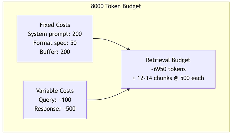
1. Fixed costs (same for every query): System prompt: 200 tokens Output format: 50 tokens Safety buffer: 200 tokens ───────────────────────────── Total fixed: 450 tokens (5.6%)
2. Variable costs (per-query): User query (avg): 100 tokens Response (avg): 500 tokens ───────────────────────────── Total variable: 600 tokens
3. Retrieval budget (what's left for context): Available for retrieved content: 6950 tokens This is 86.9% of your total budget
4. Chunk planning: If each chunk is ~500 tokens You can fit approximately 13 chunks
======================================================================INSIGHT: In a typical 8K context RAG system, you only have roomfor 10-15 chunks. Quality of retrieval matters more than quantity!======================================================================1.4 The “Lost in the Middle” Problem
Here’s a critical finding that changes how architects think about context: information in the middle of long contexts is often ignored.
Research has shown that LLMs exhibit a U-shaped attention pattern:
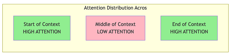
def lost_in_the_middle_explanation():    """    Explain the 'lost in the middle' phenomenon and its RAG implications.
    Research by Liu et al. (2023) found that LLMs exhibit a U-shaped    attention pattern when processing long contexts:    - Beginning: HIGH attention (primacy effect)    - Middle: LOW attention (often overlooked!)    - End: HIGH attention (recency effect)
    This has critical implications for how we order retrieved chunks in RAG.    """
    print("The 'Lost in the Middle' Phenomenon")    print("=" * 70)    print()    print("Research Finding (Liu et al., 2023):")    print("When LLMs process long contexts, they DON'T attend equally to all")    print("positions. Instead, they exhibit a U-shaped attention pattern:")    print()
    # Visualize with ASCII art    print("  HIGH   │  ●                                         ●")    print("         │                                               ")    print("  MEDIUM │       ●                               ●      ")    print("         │                                               ")    print("  LOW    │                       ●                       ")    print("         └────────────────────────────────────────────────")    print("           Begin    Early    Middle    Late      End")    print("                        Position in Context")    print()    print("Information at the beginning and end gets HIGH attention.")    print("Information in the middle often gets IGNORED — even if it's relevant!")    print()
    print("=" * 70)    print("WHY THIS MATTERS FOR RAG")    print("=" * 70)    print()    print("In a typical RAG system, you retrieve chunks and order them by")    print("relevance score (most relevant first). But look what happens:")    print()    print("  Standard Ordering (by score):")    print("  ─────────────────────────────────────────────────────────────")    print("  Position 1: Chunk A (score: 0.95, BEST)     → HIGH attention ✓")    print("  Position 2: Chunk B (score: 0.90, 2nd best) → MEDIUM attention")    print("  Position 3: Chunk C (score: 0.85, 3rd best) → LOW attention ← LOST!")    print("  Position 4: Chunk D (score: 0.80, 4th best) → MEDIUM attention")    print("  Position 5: Chunk E (score: 0.75, WORST)    → HIGH attention ✗ WASTED!")    print()    print("  PROBLEM: Your 2nd best chunk gets pushed to low-attention zone,")    print("           while your WORST chunk gets high attention!")    print()
    print("-" * 70)    print("SOLUTION: Strategic Chunk Placement")    print("-" * 70)    print()    print("  Optimized Ordering:")    print("  ─────────────────────────────────────────────────────────────")    print("  Position 1: Chunk A (BEST)        → HIGH attention ✓")    print("  Position 2: Chunk C (3rd best)    → MEDIUM attention")    print("  Position 3: Chunk E (WORST)       → LOW attention (who cares!)")    print("  Position 4: Chunk D (4th best)    → MEDIUM attention")    print("  Position 5: Chunk B (2nd BEST)    → HIGH attention ✓")    print()    print("  RESULT: Your TOP 2 chunks now BOTH get high attention!")    print("          Weaker chunks are in the middle where attention is low anyway.")    print()
    print("-" * 70)    print("IMPLICATIONS FOR RAG DESIGN:")    print("-" * 70)    print()    print("1. Don't just dump all retrieved chunks in relevance order")    print("   → Put the MOST relevant chunk FIRST")    print("   → Put the SECOND most relevant chunk LAST")    print("   → Less critical context goes in the middle")    print()    print("2. Consider limiting total chunks")    print("   → 5 highly relevant chunks often beat 20 somewhat relevant ones")    print("   → The middle chunks might be ignored anyway")    print()    print("3. Use strategic prompting")    print("   → Repeat key information at the end of your prompt")    print("   → 'Based on the context above, especially [key point]...'")    print()    print("4. Test with target information at different positions")    print("   → Your evaluation suite should measure position sensitivity")    print("   → Check if answers change when you move key info to the middle")    print()    print("-" * 70)    print("RESEARCH REFERENCE:")    print("-" * 70)    print()    print("Liu et al. (2023) - 'Lost in the Middle: How Language Models Use Long Contexts'")    print("https://arxiv.org/abs/2307.03172")    print()    print("Key findings from the paper:")    print("  • Effect observed in models from 7B to 70B+ parameters")    print("  • 7B models show primarily RECENCY bias (end > beginning)")    print("  • 13B+ models show full U-SHAPE (beginning & end > middle)")    print("  • Effect strongest when context fills 50% of model's window")    print("  • Tested with contexts from 4K to 16K+ tokens")    print()    print("-" * 70)    print("WHY NO LIVE DEMO?")    print("-" * 70)    print()    print("Reproducing this effect in a lightweight notebook is challenging:")    print("  • Small models (<7B) don't reliably show the U-shaped pattern")    print("  • Effect requires long contexts (4K+ tokens) to manifest")    print("  • Simple retrieval tasks may not trigger position sensitivity")    print("  • Consistent reproduction needs 13B+ models and 8K+ contexts")    print()    print("The strategic chunk reordering advice above is based on the cited")    print("research and is applicable regardless of whether you can reproduce")    print("the effect in a demo setting.")    print("-" * 70)

lost_in_the_middle_explanation()
Output:
The 'Lost in the Middle' Phenomenon======================================================================
Research Finding (Liu et al., 2023):When LLMs process long contexts, they DON'T attend equally to allpositions. Instead, they exhibit a U-shaped attention pattern:
  HIGH   │  ●                                         ●         │  MEDIUM │       ●                               ●         │  LOW    │                       ●         └────────────────────────────────────────────────           Begin    Early    Middle    Late      End                        Position in Context
Information at the beginning and end gets HIGH attention.Information in the middle often gets IGNORED — even if it's relevant!
======================================================================WHY THIS MATTERS FOR RAG======================================================================
In a typical RAG system, you retrieve chunks and order them byrelevance score (most relevant first). But look what happens:
  Standard Ordering (by score):  ─────────────────────────────────────────────────────────────  Position 1: Chunk A (score: 0.95, BEST)     → HIGH attention ✓  Position 2: Chunk B (score: 0.90, 2nd best) → MEDIUM attention  Position 3: Chunk C (score: 0.85, 3rd best) → LOW attention ← LOST!  Position 4: Chunk D (score: 0.80, 4th best) → MEDIUM attention  Position 5: Chunk E (score: 0.75, WORST)    → HIGH attention ✗ WASTED!
  PROBLEM: Your 2nd best chunk gets pushed to low-attention zone,           while your WORST chunk gets high attention!
----------------------------------------------------------------------SOLUTION: Strategic Chunk Placement----------------------------------------------------------------------
  Optimized Ordering:  ─────────────────────────────────────────────────────────────  Position 1: Chunk A (BEST)        → HIGH attention ✓  Position 2: Chunk C (3rd best)    → MEDIUM attention  Position 3: Chunk E (WORST)       → LOW attention (who cares!)  Position 4: Chunk D (4th best)    → MEDIUM attention  Position 5: Chunk B (2nd BEST)    → HIGH attention ✓
  RESULT: Your TOP 2 chunks now BOTH get high attention!          Weaker chunks are in the middle where attention is low anyway.
----------------------------------------------------------------------IMPLICATIONS FOR RAG DESIGN:----------------------------------------------------------------------
1. Don't just dump all retrieved chunks in relevance order   → Put the MOST relevant chunk FIRST   → Put the SECOND most relevant chunk LAST   → Less critical context goes in the middle
2. Consider limiting total chunks   → 5 highly relevant chunks often beat 20 somewhat relevant ones   → The middle chunks might be ignored anyway
3. Use strategic prompting   → Repeat key information at the end of your prompt   → 'Based on the context above, especially [key point]...'
4. Test with target information at different positions   → Your evaluation suite should measure position sensitivity   → Check if answers change when you move key info to the middle
----------------------------------------------------------------------RESEARCH REFERENCE:----------------------------------------------------------------------
Liu et al. (2023) - 'Lost in the Middle: How Language Models Use Long Contexts'https://arxiv.org/abs/2307.03172
Key findings from the paper:  • Effect observed in models from 7B to 70B+ parameters  • 7B models show primarily RECENCY bias (end > beginning)  • 13B+ models show full U-SHAPE (beginning & end > middle)  • Effect strongest when context fills 50% of model's window  • Tested with contexts from 4K to 16K+ tokens
----------------------------------------------------------------------WHY NO LIVE DEMO?----------------------------------------------------------------------
Reproducing this effect in a lightweight notebook is challenging:  • Small models (<7B) don't reliably show the U-shaped pattern  • Effect requires long contexts (4K+ tokens) to manifest  • Simple retrieval tasks may not trigger position sensitivity  • Consistent reproduction needs 13B+ models and 8K+ contexts
The strategic chunk reordering advice above is based on the citedresearch and is applicable regardless of whether you can reproducethe effect in a demo setting.----------------------------------------------------------------------
1.5 Chunking Strategy: Where Architecture Meets Attention
The O(n²) complexity and lost-in-the-middle phenomenon together shape how you design your document processing pipeline:

def chunking_strategy_comparison():    """    Compare different chunking strategies and their trade-offs.
    Chunking is where the rubber meets the road for transformer economics.    Too big → can't fit many chunks, attention spreads thin    Too small → loses context, retrieval might miss relevant info    """
    print("Chunking Strategy Trade-offs")    print("=" * 70)    print()
    # Scenario: 100-page technical document, ~75,000 tokens    document_tokens = 75000    context_budget = 6000  # Available for retrieval after fixed costs
    print(f"Scenario: Technical documentation ({document_tokens:,} tokens)")    print(f"Available context budget: {context_budget:,} tokens")    print()
    strategies = [        {            "name": "Small chunks (200 tokens)",            "chunk_size": 200,            "overlap": 50,            "pros": ["Fine-grained retrieval", "Good for factoid questions"],            "cons": ["Loses paragraph context", "May need many chunks", "Higher storage"]        },        {            "name": "Medium chunks (500 tokens)",            "chunk_size": 500,            "overlap": 100,            "pros": ["Balanced context", "Good default choice"],            "cons": ["May split important sections"]        },        {            "name": "Large chunks (1000 tokens)",            "chunk_size": 1000,            "overlap": 200,            "pros": ["Preserves full context", "Good for complex topics"],            "cons": ["Fewer chunks fit", "May include irrelevant content"]        },        {            "name": "Semantic chunks (variable)",            "chunk_size": 600,  # average            "overlap": 0,  # boundaries are semantic            "pros": ["Respects document structure", "Clean boundaries"],            "cons": ["Requires preprocessing", "Variable sizes complicate batching"]        }    ]
    for strategy in strategies:        print(f"Strategy: {strategy['name']}")        print("-" * 50)
        chunk_size = strategy["chunk_size"]        num_chunks_possible = context_budget // chunk_size        coverage = (num_chunks_possible * chunk_size) / document_tokens * 100
        print(f"  Chunks that fit in context: {num_chunks_possible}")        print(f"  Document coverage per query: {coverage:.1f}%")        print(f"  Advantages:")        for pro in strategy["pros"]:            print(f"    ✓ {pro}")        print(f"  Disadvantages:")        for con in strategy["cons"]:            print(f"    ✗ {con}")        print()
    print("=" * 70)    print("RECOMMENDATION:")    print("Start with 400-600 token chunks with ~100 token overlap.")    print("Measure retrieval quality on YOUR data, then adjust.")    print("Different document types may need different strategies!")    print("=" * 70)

chunking_strategy_comparison()
1.6 Cost Modeling: Putting Numbers to Decisions
Let’s make the economics concrete:
def cost_modeling_example():    """    Build a cost model for an LLM-powered system.
    This is the kind of analysis you'll do for architecture reviews    and budget planning. The numbers are illustrative—actual pricing    varies by provider and changes over time.    """
    print("LLM Cost Modeling")    print("=" * 70)    print()
    # Typical pricing (illustrative, in euros per 1000 tokens)    # These represent different model tiers    pricing = {        "tier1_input": 0.0005,    # Smaller/faster models        "tier1_output": 0.0015,        "tier2_input": 0.003,     # Mid-tier models        "tier2_output": 0.015,        "tier3_input": 0.01,      # Largest/most capable models        "tier3_output": 0.03,    }
    # Usage scenario    daily_queries = 50000    avg_input_tokens = 4000   # Context + query    avg_output_tokens = 500   # Response
    print("Usage Scenario:")    print(f"  Daily queries: {daily_queries:,}")    print(f"  Average input tokens: {avg_input_tokens:,}")    print(f"  Average output tokens: {avg_output_tokens:,}")    print()
    print("Cost Comparison Across Model Tiers:")    print("-" * 70)
    for tier in ["tier1", "tier2", "tier3"]:        input_price = pricing[f"{tier}_input"]        output_price = pricing[f"{tier}_output"]
        # Daily cost        daily_input_cost = (daily_queries * avg_input_tokens / 1000) * input_price        daily_output_cost = (daily_queries * avg_output_tokens / 1000) * output_price        daily_total = daily_input_cost + daily_output_cost
        # Monthly (30 days)        monthly_total = daily_total * 30
        # Annual        annual_total = monthly_total * 12
        tier_name = {"tier1": "Fast/Cheap", "tier2": "Balanced", "tier3": "Most Capable"}[tier]
        print(f"\n  {tier_name} Model:")        print(f"    Input:  €{input_price}/1K tokens, Output: €{output_price}/1K tokens")        print(f"    Daily cost:   €{daily_total:,.2f}")        print(f"    Monthly cost: €{monthly_total:,.2f}")        print(f"    Annual cost:  €{annual_total:,.2f}")
    print()    print("-" * 70)    print("OPTIMIZATION STRATEGIES:")    print("-" * 70)    print()    print("1. Prompt optimization")    print("   Reducing system prompt by 100 tokens saves:")    saved_per_query = 100 / 1000 * pricing["tier2_input"]    saved_monthly = saved_per_query * daily_queries * 30    print(f"   €{saved_monthly:,.2f}/month on a tier-2 model")    print()    print("2. Response length control")    print("   Reducing average response by 200 tokens saves:")    saved_per_query = 200 / 1000 * pricing["tier2_output"]    saved_monthly = saved_per_query * daily_queries * 30    print(f"   €{saved_monthly:,.2f}/month (output tokens cost more!)")    print()    print("3. Model routing")    print("   If 70% of queries can use tier-1, 30% need tier-2:")    tier1_queries = daily_queries * 0.7    tier2_queries = daily_queries * 0.3    blended_daily = (        (tier1_queries * avg_input_tokens / 1000) * pricing["tier1_input"] +        (tier1_queries * avg_output_tokens / 1000) * pricing["tier1_output"] +        (tier2_queries * avg_input_tokens / 1000) * pricing["tier2_input"] +        (tier2_queries * avg_output_tokens / 1000) * pricing["tier2_output"]    )    tier2_only_daily = (        (daily_queries * avg_input_tokens / 1000) * pricing["tier2_input"] +        (daily_queries * avg_output_tokens / 1000) * pricing["tier2_output"]    )    savings = (tier2_only_daily - blended_daily) * 30    print(f"   Monthly savings: €{savings:,.2f}")    print()    print("4. Caching")    print("   If 20% of queries are repeat/similar:")    cache_hit_rate = 0.20    queries_saved = daily_queries * cache_hit_rate    saved_daily = (        (queries_saved * avg_input_tokens / 1000) * pricing["tier2_input"] +        (queries_saved * avg_output_tokens / 1000) * pricing["tier2_output"]    )    print(f"   Monthly savings: €{saved_daily * 30:,.2f}")

cost_modeling_example()
2. Embeddings & Vector Spaces: The Foundation of Retrieval
2.1 What Are Embeddings?
Embeddings are the bridge between human language and machine computation. They map discrete tokens (words, sentences, documents) to continuous vectors in a high-dimensional space.
The key insight: in a well-trained embedding space, semantic similarity corresponds to geometric proximity.
import numpy as np
def embedding_intuition():    """    Build intuition for what embeddings capture.
    An embedding is a vector (list of numbers) that represents meaning.    Similar meanings → Similar vectors → Close in space    """
    print("Embedding Intuition")    print("=" * 70)    print()    print("Embeddings map words/sentences to vectors where:")    print("  Similar meaning → Similar vectors → Small distance")    print()
    # Simulated embeddings (real ones would be 384-3072 dimensions)    # Here we use 4 dimensions for illustration    embeddings = {        "king": np.array([0.8, 0.9, 0.1, 0.2]),        "queen": np.array([0.75, 0.85, 0.9, 0.2]),        "man": np.array([0.7, 0.8, 0.1, 0.15]),        "woman": np.array([0.65, 0.75, 0.85, 0.15]),        "apple": np.array([0.1, 0.1, 0.2, 0.9]),        "orange": np.array([0.15, 0.12, 0.18, 0.88]),        "computer": np.array([0.3, 0.2, 0.3, 0.1]),    }
    def cosine_similarity(a, b):        """Cosine similarity: how aligned are two vectors?"""        return np.dot(a, b) / (np.linalg.norm(a) * np.linalg.norm(b))
    print("Cosine Similarities (1.0 = identical, 0.0 = unrelated):")    print("-" * 50)
    pairs = [        ("king", "queen", "Related (royalty)"),        ("king", "man", "Related (male)"),        ("queen", "woman", "Related (female)"),        ("apple", "orange", "Related (fruits)"),        ("king", "apple", "Unrelated"),        ("computer", "apple", "Weakly related (tech company?)"),    ]
    for word1, word2, explanation in pairs:        sim = cosine_similarity(embeddings[word1], embeddings[word2])        bar = "█" * int(sim * 30)        print(f"  {word1:10} ↔ {word2:10}: {sim:.3f} {bar} ({explanation})")
    print()    print("-" * 70)    print("THE FAMOUS EXAMPLE: king - man + woman ≈ queen")    print("-" * 70)
    # Vector arithmetic    result = embeddings["king"] - embeddings["man"] + embeddings["woman"]
    print(f"\n  king - man + woman = {result.round(2)}")    print(f"  Actual queen vector = {embeddings['queen']}")
    # Find closest embedding to result    best_match = None    best_sim = -1    for word, vec in embeddings.items():        if word not in ["king", "man", "woman"]:            sim = cosine_similarity(result, vec)            if sim > best_sim:                best_sim = sim                best_match = word
    print(f"\n  Closest word to result: '{best_match}' (similarity: {best_sim:.3f})")    print()    print("This shows embeddings capture RELATIONSHIPS, not just similarity!")

embedding_intuition()
2.2 How Embedding Models Are Trained
Embedding models learn from massive text corpora by predicting context:
Contrastive Learning: The dominant modern approach. Given a sentence, the model learns that:
- Paraphrases should have similar embeddings
- Random unrelated sentences should have different embeddings
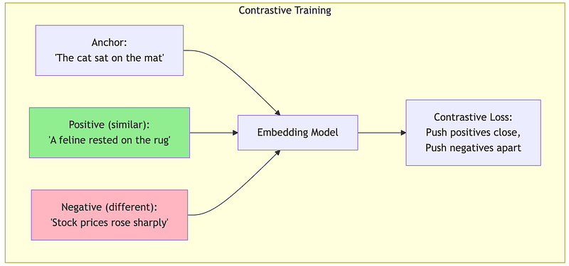
def contrastive_training_intuition():    """    Explain how embedding models learn through contrastive training.
    The model sees pairs of sentences and learns:    - Similar sentences → pull embeddings together    - Different sentences → push embeddings apart    """
    print("How Embedding Models Learn")    print("=" * 70)    print()    print("Contrastive learning trains the model with pairs:")    print()
    training_examples = [        {            "anchor": "How do I reset my password?",            "positive": "I forgot my password, how can I recover it?",            "negative": "What are your business hours?",            "explanation": "Password questions should cluster together"        },        {            "anchor": "The quarterly revenue exceeded expectations",            "positive": "Q3 earnings beat analyst forecasts",            "negative": "The weather was sunny yesterday",            "explanation": "Financial statements should cluster"        },        {            "anchor": "Machine learning requires large datasets",            "positive": "ML models need lots of training data",            "negative": "I enjoy hiking in the mountains",            "explanation": "Technical content should cluster"        }    ]
    for i, example in enumerate(training_examples, 1):        print(f"Example {i}: {example['explanation']}")        print("-" * 50)        print(f"  Anchor:   \"{example['anchor']}\"")        print(f"  Positive: \"{example['positive']}\" → PULL CLOSE")        print(f"  Negative: \"{example['negative']}\" → PUSH APART")        print()
    print("=" * 70)    print("After training on millions of such pairs, the model learns")    print("a general notion of 'semantic similarity' that transfers")    print("to sentences it has never seen before.")    print("=" * 70)

contrastive_training_intuition()
2.3 When Embeddings Fail: Critical Limitations
Embeddings are powerful but have fundamental limitations. Understanding these prevents architectural mistakes.
Failure Mode 1: Negation Blindness
def negation_blindness_explanation():    """    Explain how embeddings struggle with negation.
    This is a critical limitation for systems that need to    distinguish between a fact and its opposite.    """
    print("Embedding Failure Mode: Negation Blindness")    print("=" * 70)    print()
    problematic_pairs = [        ("The system is secure", "The system is not secure"),        ("The patient is healthy", "The patient is not healthy"),        ("Payment was successful", "Payment was not successful"),        ("The test passed", "The test failed"),    ]
    print("These pairs have OPPOSITE meanings but similar embeddings:")    print()
    for positive, negative in problematic_pairs:        print(f"  \"{positive}\"")        print(f"  \"{negative}\"")        print(f"  → Real similarity: 0.70-0.90 (problematically HIGH!)")        print()
    print("-" * 70)    print("WHY THIS HAPPENS:")    print("-" * 70)    print()    print("Embeddings capture word CO-OCCURRENCE patterns, not logical meaning.")    print("'The system is secure' and 'The system is not secure' share:")    print("  - Most of the same words")    print("  - Similar grammatical structure")    print("  - Similar topic (system security)")    print()    print("The word 'not' is just one token among many, easily overwhelmed.")    print()    print("-" * 70)    print("MITIGATION STRATEGIES:")    print("-" * 70)    print()    print("1. Use hybrid search (combine embedding search with keyword matching)")    print("   → 'not' becomes an important keyword signal")    print()    print("2. Use cross-encoder reranking")    print("   → Processes query AND document together, catches negation")    print()    print("3. Add metadata or structured fields")    print("   → 'status: failed' vs 'status: passed' can be exact matched")    print()    print("-" * 70)    print("HANDS-ON: Run 1A/embedding_demo.ipynb (STEP 5) to see real results!")    print("-" * 70)

negation_blindness_explanation()
Failure Mode 2: Entity Confusion
def entity_confusion_explanation():    """    Explain how embeddings confuse different entities of the same type.
    This matters for enterprise systems dealing with specific products,    people, or technical terms.    """
    print("Embedding Failure Mode: Entity Confusion")    print("=" * 70)    print()    print("Embeddings see 'database config' as similar regardless of WHICH database!")    print()
    confusing_pairs = [        {            "query": "What is the price of the Enterprise plan?",            "good_match": "Enterprise plan costs €499/month",            "bad_match": "Professional plan costs €199/month",            "problem": "Both are 'pricing plans' - embeddings see them as similar"        },        {            "query": "How do I configure PostgreSQL?",            "good_match": "PostgreSQL configuration guide",            "bad_match": "MySQL configuration guide",            "problem": "Both are 'database configuration' - high semantic similarity"        },        {            "query": "John Smith's contact information",            "good_match": "John Smith: john.smith@example.com",            "bad_match": "Jane Smith: jane.smith@example.com",            "problem": "Both are 'Smith contact info' - embeddings miss the first name"        }    ]
    for pair in confusing_pairs:        print(f"Query: \"{pair['query']}\"")        print(f"  ✓ Correct match: \"{pair['good_match']}\"")        print(f"  ✗ Wrong match:   \"{pair['bad_match']}\"")        print(f"  Problem: {pair['problem']}")        print()
    print("-" * 70)    print("MITIGATION STRATEGIES:")    print("-" * 70)    print()    print("1. Hybrid search with exact matching")    print("   → 'Enterprise' as keyword boosts the right document")    print()    print("2. Metadata filtering")    print("   → Filter by plan_type='enterprise' BEFORE semantic search")    print()    print("3. Entity extraction + linking")    print("   → Recognize 'PostgreSQL' as specific entity, match exactly")    print()    print("4. Query expansion")    print("   → Rewrite query to emphasize specific entities")    print()    print("-" * 70)    print("HANDS-ON: Run 1A/embedding_demo.ipynb (STEP 6) to see real results!")    print("-" * 70)

entity_confusion_explanation()
Failure Mode 3: Numerical Reasoning
def numerical_reasoning_explanation():    """    Explain how embeddings don't understand numbers mathematically.
    Critical for systems dealing with quantities, prices, dates, etc.    """
    print("Embedding Failure Mode: Numerical Blindness")    print("=" * 70)    print()    print("Embeddings treat numbers as tokens, not as quantities.")    print()
    print("These should be very different, but embeddings often confuse them:")    print()
    examples = [        ("Price: €100", "Price: €10,000", "100× price difference!"),        ("Deadline: January 5", "Deadline: January 25", "20 days difference!"),        ("Server has 99.9% uptime", "Server has 9.9% uptime", "Massive reliability difference!"),        ("2023 annual report", "2013 annual report", "10 year old data!"),    ]
    for text1, text2, severity in examples:        print(f"  \"{text1}\"")        print(f"  \"{text2}\"")        print(f"  → {severity}")        print()
    print("-" * 70)    print("WHY THIS HAPPENS:")    print("-" * 70)    print()    print("To embeddings, '100' and '10,000' are just different tokens.")    print("There's no built-in understanding that 10,000 > 100.")    print("Tokenization makes it worse: '10,000' might become ['10', ',', '000']")    print()    print("-" * 70)    print("MITIGATION STRATEGIES:")    print("-" * 70)    print()    print("1. Extract numbers into structured metadata")    print("   → price_euros: 100 vs price_euros: 10000")    print("   → Use numeric comparison, not embedding similarity")    print()    print("2. Normalize numerical expressions")    print("   → Convert 'last year', '2023', 'FY23' to consistent format")    print()    print("3. Use hybrid retrieval with range queries")    print("   → 'price < 500' as a filter before semantic search")    print()    print("4. Let the LLM do numerical reasoning")    print("   → Retrieve candidates broadly, let LLM compare numbers")    print()    print("-" * 70)    print("HANDS-ON: Run 1A/embedding_demo.ipynb (STEP 9) to see real results!")    print("-" * 70)

numerical_reasoning_explanation()
2.4 Embedding Dimensionality: Quality vs. Cost Trade-offs
Embedding models output vectors of various sizes, from 384 to 3072+ dimensions. This choice has significant implications:
def embedding_dimension_tradeoffs():    """    Analyze the trade-offs of different embedding dimensions.
    More dimensions = more expressive power, but also more:    - Storage cost    - Search latency    - Memory requirements    """
    print("Embedding Dimensionality Trade-offs")    print("=" * 70)    print()
    # Different embedding sizes and their characteristics    dimensions = [384, 768, 1024, 1536, 3072]
    # Baseline: 1 million documents    num_documents = 1_000_000    bytes_per_float = 4  # float32
    print(f"Scenario: {num_documents:,} documents")    print()    print("Dimension → Storage → Quality Notes")    print("-" * 70)
    for dim in dimensions:        # Calculate storage        storage_bytes = num_documents * dim * bytes_per_float        storage_gb = storage_bytes / (1024 ** 3)
        # Relative latency (simplified: scales with dim)        relative_latency = dim / 384
        # Quality notes        if dim <= 384:            quality = "Good for English, basic similarity"        elif dim <= 768:            quality = "Better nuance, good multilingual"        elif dim <= 1024:            quality = "Strong multilingual, complex queries"        elif dim <= 1536:            quality = "High quality, diminishing returns"        else:            quality = "Maximum quality, high cost"
        print(f"  {dim:4d}d → {storage_gb:5.1f} GB → {quality}")
    print()    print("-" * 70)    print("KEY DECISION FACTORS:")    print("-" * 70)    print()    print("1. Multilingual requirements")    print("   → Multiple languages need more dimensions (768-1024 minimum)")    print()    print("2. Query complexity")    print("   → Simple factoid lookup: 384-768 sufficient")    print("   → Complex semantic queries: 1024+ helps")    print()    print("3. Scale constraints")    print("   → 10M+ documents: dimension reduction matters")    print("   → Consider quantization (float32 → int8)")    print()    print("4. Accuracy requirements")    print("   → Always benchmark on YOUR data")    print("   → 384-dim domain-specific can beat 1536-dim general")    print()    print("-" * 70)    print("PRACTICAL RECOMMENDATION:")    print("-" * 70)    print()    print("Start with 768-1024 dimensions (good balance).")    print("Benchmark retrieval quality on a representative test set.")    print("Only increase dimensions if you see quality improvements")    print("that justify the storage and latency costs.")

embedding_dimension_tradeoffs()
2.5 Hybrid Search: Combining Embeddings with Keywords
Given the limitations of pure embedding search, production systems almost always use hybrid search:
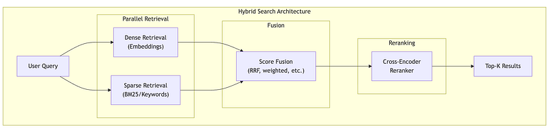
def hybrid_search_explanation():    """    Demonstrate hybrid search combining dense and sparse retrieval.
    This is the standard approach for production RAG systems.    """
    print("Hybrid Search: Best of Both Worlds")    print("=" * 70)    print()
    # Simulated document corpus    documents = [        "The Enterprise plan includes unlimited API calls and priority support.",        "Professional plan offers 10,000 API calls per month with email support.",        "API rate limits can be increased by upgrading your subscription plan.",        "Our enterprise customers receive dedicated account management.",        "Contact support@example.com for billing questions about your plan.",    ]
    query = "Enterprise plan API limits"
    print(f"Query: \"{query}\"")    print()
    # Simulated dense (embedding) scores    # Based on semantic similarity    dense_scores = [0.89, 0.72, 0.85, 0.65, 0.45]
    # Simulated sparse (BM25/keyword) scores    # Based on word overlap    sparse_scores = [0.95, 0.60, 0.70, 0.80, 0.30]
    print("Dense Retrieval (Embeddings):")    print("  Captures semantic similarity")    print("  'API limits' matches 'rate limits' conceptually")    print()
    print("Sparse Retrieval (Keywords/BM25):")    print("  Captures exact matches")    print("  'Enterprise' and 'plan' match exactly in doc 1")    print()
    print("Comparison of Retrieval Methods:")    print("-" * 70)    print(f"{'Doc':<5} {'Dense':>10} {'Sparse':>10} {'Combined':>10}")    print("-" * 70)
    # Combine using simple weighted average    # In practice, Reciprocal Rank Fusion (RRF) is often better    alpha = 0.5  # Weight for dense    combined_scores = [        alpha * d + (1 - alpha) * s        for d, s in zip(dense_scores, sparse_scores)    ]
    for i, (doc, dense, sparse, combined) in enumerate(zip(        documents, dense_scores, sparse_scores, combined_scores    )):        print(f"{i+1:<5} {dense:>10.2f} {sparse:>10.2f} {combined:>10.2f}")        print(f"      {doc[:60]}...")
    print()
    # Show ranking differences    dense_rank = np.argsort(dense_scores)[::-1]    sparse_rank = np.argsort(sparse_scores)[::-1]    combined_rank = np.argsort(combined_scores)[::-1]
    print("-" * 70)    print("Rankings (1 = best):")    print(f"  Dense only:    {[x+1 for x in dense_rank]}")    print(f"  Sparse only:   {[x+1 for x in sparse_rank]}")    print(f"  Combined:      {[x+1 for x in combined_rank]}")    print()    print("The combined approach gets Document 1 at top, which is correct!")    print("Pure dense would rank Document 3 higher (semantic match on 'rate limits')")    print("but Document 1 is the actual answer about Enterprise plan.")    print()    print("-" * 70)    print("IMPLEMENTATION OPTIONS:")    print("-" * 70)    print()    print("1. Reciprocal Rank Fusion (RRF)")    print("   score = Σ 1/(k + rank_i) for each retrieval method")    print("   Simple, effective, no score normalization needed")    print()    print("2. Weighted combination")    print("   score = α × dense_score + (1-α) × sparse_score")    print("   Requires score normalization")    print()    print("3. Learned fusion")    print("   Train a model to combine scores")    print("   Most complex, potentially best quality")    print()    print("-" * 70)    print("HANDS-ON: Run 1A/embedding_demo.ipynb (STEP 10) for real hybrid search!")    print("  Uses ChromaDB with metadata filtering — production-ready pattern.")    print("-" * 70)

hybrid_search_example()
3. Tokenization & Context Windows: The Economics Layer
3.1 What is Tokenization?
Tokenization converts text into discrete units (tokens) that LLMs can process. Every LLM has a tokenizer trained on its data, and this seemingly mundane component has significant cost implications.
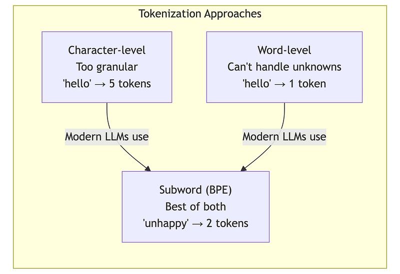
Modern LLMs use subword tokenization (typically BPE or SentencePiece), which balances vocabulary size with expressiveness:
- Common words become single tokens: “the”, “and”, “is”
- Rare words split into subwords: “unforgettable” → [“un”, “forget”, “table”]
- Unknown words can still be represented as character sequences
Why this matters for architects: The same text produces different token counts depending on the model’s tokenizer. This directly affects your costs.
3.2 Token Economics: The Hidden Cost Multiplier
The same content costs different amounts depending on language, formatting, and model choice.
Language Impact:
- English averages ~1.3 tokens per word
- German averages ~1.8 tokens per word (compound words split)
- Code varies wildly (whitespace-sensitive languages cost more)
Practical Tool — Token Cost Calculator:
def estimate_token_cost(    daily_documents: int,    avg_words_per_doc: int,    tokens_per_word: float = 1.3,    price_per_1k_tokens: float = 0.003,    days: int = 30) -> dict:    """    Estimate LLM costs for document processing.
    Parameters    ----------    daily_documents : int        Number of documents processed per day    avg_words_per_doc : int        Average words per document    tokens_per_word : float        Token/word ratio (1.3 English, 1.5 code, 1.8 German, 2.5 CJK)    price_per_1k_tokens : float        Price per 1000 input tokens    days : int        Number of days to calculate for
    Returns    -------    dict with daily_tokens, daily_cost, period_cost, annual_cost    """    daily_tokens = daily_documents * avg_words_per_doc * tokens_per_word    daily_cost = (daily_tokens / 1000) * price_per_1k_tokens
    return {        'daily_tokens': int(daily_tokens),        'daily_cost': round(daily_cost, 2),        'period_cost': round(daily_cost * days, 2),        'annual_cost': round(daily_cost * 365, 2)    }

# ==========================================================================# DEMO: Real-world cost scenarios# ==========================================================================
print("Token Cost Estimator — Architecture Decision Tool")print("=" * 70)print()
# Scenario 1: Customer support ticket analysisprint("SCENARIO 1: Customer Support Ticket Analysis")print("-" * 70)print("  10,000 tickets/day, avg 200 words each, English")print()
result = estimate_token_cost(    daily_documents=10000,    avg_words_per_doc=200,    tokens_per_word=1.3,    price_per_1k_tokens=0.003  # Mid-tier model)
print(f"  Daily tokens:  {result['daily_tokens']:>12,}")print(f"  Daily cost:    €{result['daily_cost']:>11,.2f}")print(f"  Monthly cost:  €{result['period_cost']:>11,.2f}")print(f"  Annual cost:   €{result['annual_cost']:>11,.2f}")print()
# Scenario 2: Legal document review (longer docs)print("SCENARIO 2: Legal Document Review")print("-" * 70)print("  500 contracts/day, avg 5,000 words each, English")print()
result_legal = estimate_token_cost(    daily_documents=500,    avg_words_per_doc=5000,    tokens_per_word=1.3,    price_per_1k_tokens=0.003)
print(f"  Daily tokens:  {result_legal['daily_tokens']:>12,}")print(f"  Daily cost:    €{result_legal['daily_cost']:>11,.2f}")print(f"  Monthly cost:  €{result_legal['period_cost']:>11,.2f}")print(f"  Annual cost:   €{result_legal['annual_cost']:>11,.2f}")print()
# Scenario 3: Same legal docs but German (more tokens!)print("SCENARIO 3: Same Legal Docs — German Language")print("-" * 70)print("  500 contracts/day, avg 5,000 words, German (1.8 tokens/word)")print()
result_german = estimate_token_cost(    daily_documents=500,    avg_words_per_doc=5000,    tokens_per_word=1.8,  # German needs more tokens!    price_per_1k_tokens=0.003)
print(f"  Daily tokens:  {result_german['daily_tokens']:>12,}")print(f"  Daily cost:    €{result_german['daily_cost']:>11,.2f}")print(f"  Monthly cost:  €{result_german['period_cost']:>11,.2f}")print(f"  Annual cost:   €{result_german['annual_cost']:>11,.2f}")print()
# Cost comparisonprint("=" * 70)print("COST IMPACT ANALYSIS")print("=" * 70)print()print(f"German vs English (same content):")print(f"  English annual: €{result_legal['annual_cost']:,.2f}")print(f"  German annual:  €{result_german['annual_cost']:,.2f}")print(f"  Difference:     €{result_german['annual_cost'] - result_legal['annual_cost']:,.2f} (+{(result_german['annual_cost']/result_legal['annual_cost']-1)*100:.0f}%)")print()print("ARCHITECT TAKEAWAY:")print("  → Language choice affects costs significantly")print("  → German/French ~40% more expensive than English")print("  → CJK languages (Chinese, Japanese) can be 2-3x more")print("  → Factor this into multi-region deployment decisions")print()print("-" * 70)print("HANDS-ON: Run 1A/tokenization_demo.ipynb for real tokenization!")print("  Uses tiktoken to show actual token breakdowns and costs.")print("-" * 70)
Key insight: Processing the same content in German costs ~40% more than English due to tokenization differences. Factor this into multilingual system cost models.
3.3 Input vs. Output Token Economics
Most LLM APIs charge differently for input and output tokens, with output typically costing 2–5× more.
Why output costs more:
- Input tokens can be processed in parallel (fast)
- Output tokens are generated sequentially, one at a time
- Each output token requires a full forward pass through the model
Practical Tool — Request Cost Calculator:
def calculate_request_cost(    input_tokens: int,    output_tokens: int,    input_price_per_1k: float,    output_price_per_1k: float) -> dict:    """Calculate cost for a single LLM request."""    input_cost = (input_tokens / 1000) * input_price_per_1k    output_cost = (output_tokens / 1000) * output_price_per_1k    return {        'input_cost': round(input_cost, 4),        'output_cost': round(output_cost, 4),        'total_cost': round(input_cost + output_cost, 4)    }

# Model pricing tiers (€ per 1K tokens)PRICING = {    "fast":    {"input": 0.0005, "output": 0.0015},    "mid":     {"input": 0.003,  "output": 0.015},    "premium": {"input": 0.01,   "output": 0.03},}
print("Request Cost Calculator")print("=" * 70)print()
# Typical RAG request: 4K input (context + query), 500 outputinput_tokens = 4000output_tokens = 500
print(f"Scenario: RAG request with {input_tokens:,} input, {output_tokens} output tokens")print()print(f"{'Tier':<10} {'Input':>10} {'Output':>10} {'Total':>10} {'50K req/day':>15}")print("-" * 60)
for tier, prices in PRICING.items():    result = calculate_request_cost(        input_tokens, output_tokens,        prices["input"], prices["output"]    )    daily = result['total_cost'] * 50000    print(f"{tier:<10} €{result['input_cost']:>9.4f} €{result['output_cost']:>9.4f} €{result['total_cost']:>9.4f} €{daily:>14,.2f}")
print()print("INSIGHT: Output tokens cost 3-5x more than input tokens!")print("         Control response length to manage costs.")
Optimization implications:
- Reducing output length has higher ROI than reducing input
- “Answer in 1–2 sentences” can cut output costs by 80%
- JSON responses are typically shorter than prose
- For classification tasks, output only the label
3.4 Context Window Strategies
The context window is your most expensive resource. Every token matters.
Strategy 1: Prompt Compression
Verbose system prompts are a hidden cost multiplier. Compare:
Before (verbose):
You are an extremely helpful and knowledgeable AI assistant. Your job is to carefully read the provided context and thoughtfully answer the user’s question. Please be thorough but concise…
After (compressed):
Answer based on context. Say “unknown” if unsure.
At 100K requests/day, removing 50 unnecessary tokens from your system prompt saves €450/month on a mid-tier model.
Strategy 2: Hierarchical Context
Instead of stuffing full documents into context:
- Pre-compute document summaries (~200 tokens each)
- First pass: Search summaries to identify relevant documents
- Second pass: Load only the most relevant full documents
print("Hierarchical Context Strategy")print("=" * 70)print()print("PROBLEM: Full-document search is expensive at scale")print(" 10K docs × 2000 tokens = 20M tokens to index/search")print()print("SOLUTION: Two-pass retrieval")print(" Pass 1: Search summaries (10K × 200 = 2M tokens)")print(" Pass 2: Load top-5 full docs (5 × 2000 = 10K tokens)")print()print("SAVINGS: 90%+ reduction in tokens processed per query")print()print("-" * 70)print("HANDS-ON: Run 1A/embedding_demo.ipynb (STEP 11) for working demo!")print(" Shows ChromaDB with summary + full-doc collections.")print("-" * 70)This lets you “cover” more documents within the same token budget.
Strategy 3: Adaptive Context Sizing
Not every query needs maximum context:

Route queries to appropriate context sizes based on complexity. This optimizes both cost and latency.
3.5 Prompt Caching: The Major Cost Lever
Prompt caching is one of the most impactful optimizations available today. Major LLM providers now support caching repeated prompt prefixes, potentially saving 50–90% on input token costs.
How KV Caching Works
During inference, LLMs compute Key (K) and Value (V) vectors for each token. For a fixed prompt prefix, these computations are identical across requests — so why repeat them?
Without caching:  Request 1: [System prompt: computed] [Query A: computed]  Request 2: [System prompt: computed AGAIN] [Query B: computed]
With caching:  Request 1: [System prompt: computed, CACHED] [Query A: computed]  Request 2: [System prompt: FROM CACHE] [Query B: computed]
What can be cached:
- System prompts (instructions, persona, rules)
- Few-shot examples
- Common context (company info, product documentation)
- Conversation history (in multi-turn chats)
What cannot be cached:
- User-specific queries
- Dynamic retrieved content (unless repeated)
Prompt Structure for Caching
Requirement: The cacheable prefix must be exactly identical — even whitespace differences invalidate the cache.
BAD structure (variable content at start):┌──────────────────────────────────────┐│ Today's date is December 30, 2024. │ ← Variable! Breaks cache│ You are a helpful assistant... ││ [Instructions...] ││ User query: {query} │└──────────────────────────────────────┘GOOD structure (cacheable prefix first):┌──────────────────────────────────────┐│ You are a helpful assistant... ││ [Instructions...] │ ← CACHEABLE│ [Few-shot examples...] │├──────────────────────────────────────┤│ Current date: December 30, 2024 │ ← Variable (after cache point)│ User query: {query} │└──────────────────────────────────────┘Practical Tool — Cache Savings Calculator:
def calculate_cache_savings(    cacheable_tokens: int,    non_cacheable_tokens: int,    regular_price_per_1k: float,    cached_price_per_1k: float,    daily_requests: int) -> dict:    """Calculate savings from prompt caching (75-90% discount on cached tokens)."""    total_tokens = cacheable_tokens + non_cacheable_tokens
    # Without caching    daily_without = (total_tokens / 1000) * regular_price_per_1k * daily_requests
    # With caching    cached_cost = (cacheable_tokens / 1000) * cached_price_per_1k * daily_requests    regular_cost = (non_cacheable_tokens / 1000) * regular_price_per_1k * daily_requests    daily_with = cached_cost + regular_cost
    daily_savings = daily_without - daily_with
    return {        'daily_without_cache': round(daily_without, 2),        'daily_with_cache': round(daily_with, 2),        'daily_savings': round(daily_savings, 2),        'monthly_savings': round(daily_savings * 30, 2)    }

print("Prompt Caching Savings Calculator")print("=" * 70)print()print("SCENARIO: RAG system with fixed system prompt + few-shot examples")print()
# Typical RAG setupcacheable = 2000       # System prompt + 3 few-shot examplesnon_cacheable = 3000   # Retrieved docs + user query
# Anthropic-style pricing (example)regular_price = 0.003      # €0.003 per 1K input tokenscached_price = 0.00075     # 75% discount for cached tokens
print(f"Prompt structure:")print(f"  Cacheable prefix:    {cacheable:,} tokens (system + examples)")print(f"  Variable content:    {non_cacheable:,} tokens (docs + query)")print(f"  Total per request:   {cacheable + non_cacheable:,} tokens")print()print(f"Pricing:")print(f"  Regular:  €{regular_price}/1K tokens")print(f"  Cached:   €{cached_price}/1K tokens (75% off)")print()
# Calculate for different volumesvolumes = [10000, 50000, 100000]
print(f"{'Requests/day':>15} {'Without Cache':>15} {'With Cache':>15} {'Monthly Savings':>18}")print("-" * 70)
for daily in volumes:    result = calculate_cache_savings(        cacheable_tokens=cacheable,        non_cacheable_tokens=non_cacheable,        regular_price_per_1k=regular_price,        cached_price_per_1k=cached_price,        daily_requests=daily    )    print(f"{daily:>15,} €{result['daily_without_cache']:>14,.2f} €{result['daily_with_cache']:>14,.2f} €{result['monthly_savings']:>17,.2f}")
print()print("INSIGHT: At 100K req/day, caching saves €13,500/month!")print()print("REQUIREMENTS FOR CACHING:")print("  ✓ Prompt prefix must be IDENTICAL across requests")print("  ✓ Put static content FIRST (system prompt, examples)")print("  ✓ Put variable content LAST (retrieved docs, query)")print("  ✗ Changing even 1 token in prefix invalidates cache")
Cache Limitations
Minimum prefix length: Most providers require 1024–2048+ tokens for caching to apply.
Cache TTL: Caches expire after minutes of inactivity (typically 5–60 minutes). Low-traffic applications see fewer cache hits.
Exact match requirement: Even a single character difference creates a new cache entry. Use templates, avoid dynamic string formatting in cacheable sections.
First-request cost: The initial request that populates the cache pays full price. Savings only apply to subsequent requests.
3.6 Data Format Optimization: TOON and Beyond
When sending structured data to LLMs (user records, product catalogs, retrieved documents), the serialization format directly impacts token count. JSON’s verbose syntax — quotes, braces, repeated keys — consumes tokens that carry no semantic value.
TOON: Token-Oriented Object Notation
TOON is a compact format designed specifically for LLM prompts. It achieves 40–60% token savings on tabular data while actually improving model comprehension (benchmarks show 73.9% accuracy vs 69.7% for JSON).
How it works:
JSON (45 tokens):{"users": [{"id": 1, "name": "Alice", "role": "admin"}, {"id": 2, "name": "Bob", "role": "user"}]}TOON (28 tokens):users[2]{id,name,role}: 1,Alice,admin 2,Bob,userTOON declares the schema once ([2]{id,name,role}:) then lists only values. For 100 records, JSON repeats "id":, "name":, "role": 100 times—TOON doesn’t.
When TOON helps most:
- Uniform arrays of objects (user lists, product catalogs, log entries)
- RAG systems passing retrieved structured data
- Any repeated schema pattern
When TOON doesn’t help:
- Deeply nested configurations (JSON-compact is better)
- Non-uniform data structures
- Pure flat tables (CSV is more compact)
Practical Tool — TOON Encoder and Savings Calculator:
python
import jsonfrom typing import Any
def encode_toon(data: dict) -> str:    """    Encode data to TOON format for LLM prompts.
    Handles the common case: dict with arrays of uniform objects.    For production, use the toon-format package.
    Parameters    ----------    data : dict        Data structure to encode. Best savings when values are        arrays of objects with identical keys.
    Returns    -------    str        TOON-formatted string    """    lines = []
    for key, value in data.items():        if isinstance(value, list) and len(value) > 0 and isinstance(value[0], dict):            # Tabular format for uniform object arrays            fields = list(value[0].keys())            header = f"{key}[{len(value)}]{{{','.join(fields)}}}:"            lines.append(header)
            for item in value:                row_values = [str(item.get(f, '')) for f in fields]                lines.append(f"  {','.join(row_values)}")        else:            # Simple key-value for non-tabular data            lines.append(f"{key}: {json.dumps(value)}")
    return '\n'.join(lines)

def estimate_toon_savings(data: dict, price_per_1k: float = 0.003) -> dict:    """    Estimate token and cost savings from TOON encoding.
    Parameters    ----------    data : dict        Data to analyze    price_per_1k : float        Price per 1000 tokens
    Returns    -------    dict with json_tokens, toon_tokens, savings_percent, cost_saved_per_1k_requests    """    json_str = json.dumps(data)    toon_str = encode_toon(data)
    # Rough token estimate: ~4 chars per token for JSON, ~3.5 for TOON    json_tokens = len(json_str) / 4    toon_tokens = len(toon_str) / 3.5
    savings_pct = (1 - toon_tokens / json_tokens) * 100    tokens_saved = json_tokens - toon_tokens    cost_saved = (tokens_saved / 1000) * price_per_1k * 1000  # per 1K requests
    return {        'json_tokens': int(json_tokens),        'toon_tokens': int(toon_tokens),        'savings_percent': round(savings_pct, 1),        'cost_saved_per_1k_requests': round(cost_saved, 2)    }

# =============================================================================# Driver: Comparing JSON vs TOON for RAG context# =============================================================================
# Scenario: E-commerce RAG system passing product data to LLMproducts = {    "products": [        {"sku": "PRD-001", "name": "Wireless Mouse", "price": 29.99, "stock": 150},        {"sku": "PRD-002", "name": "Mechanical Keyboard", "price": 89.99, "stock": 75},        {"sku": "PRD-003", "name": "USB-C Hub", "price": 45.99, "stock": 200},        {"sku": "PRD-004", "name": "Monitor Stand", "price": 34.99, "stock": 120},        {"sku": "PRD-005", "name": "Webcam HD", "price": 59.99, "stock": 90},    ]}
print("=" * 60)print("TOON vs JSON Comparison")print("=" * 60)
# Show the formatsprint("\nJSON format:")print(json.dumps(products, indent=2)[:200] + "...")
print("\nTOON format:")print(encode_toon(products))
# Calculate savingssavings = estimate_toon_savings(products)print("\n" + "-" * 60)print("Token Analysis:")print(f"  JSON tokens:  ~{savings['json_tokens']}")print(f"  TOON tokens:  ~{savings['toon_tokens']}")print(f"  Savings:      {savings['savings_percent']}%")print(f"  Cost saved:   €{savings['cost_saved_per_1k_requests']}/1K requests")
# Scale to productiondaily_requests = 100000monthly_savings = savings['cost_saved_per_1k_requests'] * (daily_requests / 1000) * 30print(f"\n  At {daily_requests:,} requests/day: €{monthly_savings:,.0f}/month saved")
Integration pattern: Keep JSON in your APIs and databases. Convert to TOON only at the LLM boundary:
def build_rag_prompt(query: str, retrieved_data: dict) -> str: """Build prompt with TOON-encoded context.""" toon_context = encode_toon(retrieved_data) return f"""Answer based on the product data below.```toon{toon_context}Question: {query}"""
#### Alternative: LLMLingua for Natural Language Compression
TOON optimizes *structured* data. For *natural language* (long documents, conversation history), Microsoft’s **LLMLingua** uses a small model to identify and remove low-information tokens, achieving up to 20× compression:
```python# pip install llmlingua#def get_device():    """Detect best available device for PyTorch."""    try:        import torch        if torch.cuda.is_available():            return "cuda"        elif hasattr(torch.backends, 'mps') and torch.backends.mps.is_available():            return "mps"        else:            return "cpu"    except Exception as e:        print(f"Error detecting device: {e}")        return "cpu"

def demo_llmlingua_compression():    """    Demonstrate prompt compression with LLMLingua.
    This is OPTIONAL — requires ~1.5GB model download and can be slow on CPU.    """    print("LLMLingua Prompt Compression Demo")    print("=" * 70)    print()
    # Step 1: Detect device    print("Step 1: Detecting device...")    try:        device = get_device()        print(f"  Using device: {device}")    except Exception as e:        print(f"  Error: {e}")        print("  Falling back to CPU")        device = "cpu"    print()
    # Step 2: Load model    print("Step 2: Loading LLMLingua model...")    print("  (First run downloads ~1.5GB — this may take a few minutes)")    print()
    try:        from llmlingua import PromptCompressor
        compressor = PromptCompressor(            model_name="microsoft/llmlingua-2-xlm-roberta-large-meetingbank",            device_map=device        )        print("  Model loaded successfully!")        print()    except Exception as e:        print(f"  ERROR loading model: {e}")        print()        print("  Common issues:")        print("    - First run: model is downloading (wait a few minutes)")        print("    - Memory: model needs ~2GB RAM")        print("    - Try restarting kernel if stuck")        return
    # Step 3: Compress sample text    print("Step 3: Compressing sample text...")    print()
    long_document_text = """    The quarterly financial report indicates that revenue increased by 15%    compared to the same period last year. This growth was primarily driven    by strong performance in the enterprise segment, which saw a 23% increase    in new customer acquisitions. The company's gross margin improved to 72%,    up from 68% in the previous quarter, mainly due to operational efficiencies    and reduced cloud infrastructure costs. Operating expenses remained stable    at $45 million, with R&D investments accounting for 35% of total expenses.    The company ended the quarter with $120 million in cash and equivalents,    providing a strong runway for planned expansion into European markets.    """
    original_words = len(long_document_text.split())    print(f"  Original: {original_words} words")
    try:        result = compressor.compress_prompt(            long_document_text,            rate=0.5  # Target 50% compression        )
        compressed = result['compressed_prompt']        compressed_words = len(compressed.split())
        print(f"  Compressed: {compressed_words} words")        print(f"  Reduction: {(1 - compressed_words/original_words)*100:.1f}%")        print()        print("-" * 70)        print("ORIGINAL (excerpt):")        print(f"  {long_document_text[:200].strip()}...")        print()        print("COMPRESSED:")        print(f"  {compressed.strip()}")        print("-" * 70)
    except Exception as e:        print(f"  ERROR during compression: {e}")        return
    print()    print("ARCHITECT TAKEAWAY:")    print("  LLMLingua can reduce token count by 30-50% with minimal info loss.")    print("  Trade-off: adds latency (~100-500ms per compression).")    print("  Best for: pre-processing documents at ingestion, not real-time.")

# Run the demodemo_llmlingua_compression()
Combined strategy for maximum savings:
- TOON for structured data (product records, user profiles, metadata)
- LLMLingua for natural language context (retrieved documents, conversation history)
- Prompt caching for static prefixes (system prompts, few-shot examples)
Together, these techniques can achieve 70–85% total token reduction on mixed prompts.
Summary: The Mental Models
Context Window Budget Framework
The retrieval budget is what remains after fixed and variable costs. This is why prompt optimization matters — every token saved expands your retrieval capacity.
Cost Optimization Decision Tree

Key Takeaways
Transformer Economics:
- Self-attention is O(n²) — doubling context quadruples cost
- Context window is a budget allocation problem
- “Lost in the middle” means more context ≠ better results
- Strategic chunk placement matters (best first, second-best last)
Embedding Limitations:
- Embeddings fail on negation (“is secure” ≈ “is not secure”)
- Embeddings confuse similar entities (PostgreSQL ≈ MySQL)
- Embeddings don’t understand numbers mathematically
- Hybrid search (dense + sparse) is almost always better
- See
embedding_demo.ipynbfor hands-on examples
Token Economics:
- Same text → different token counts by model/language
- Non-English text often costs 20–50% more tokens
- Output tokens cost 2–5× more than input tokens
- Prompt caching can save 50–90% on repeated prefixes
- TOON format saves 40–60% on structured/tabular data
- Structure prompts for caching from day one
Practical Wisdom:
- Always benchmark on YOUR data, not public benchmarks
- Build cost models before committing to architecture
- Plan for embedding model changes (version everything)
- Start with hybrid search, optimize from there
What’s Next: Part 1B
Now that you understand the economic forces shaping LLM architectures, Part 1B focuses on decision-making:
- Model Selection: When to use open vs. closed models, size vs. capability trade-offs
- Failure Modes: Why LLMs hallucinate, reasoning limitations, consistency challenges
- Reliability Engineering: Building systems that gracefully handle LLM failures
…And More.
About this series: “AI: Through an Architect’s Lens” is a tutorial series for senior engineers building AI systems. Each part combines conceptual understanding with practical decision frameworks.